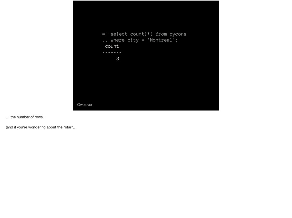
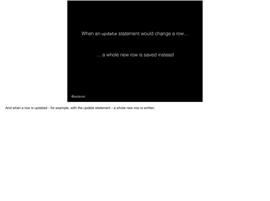
(1 row) In this talk I’m going to be talking about COUNT(*) COUNT(*) is the SQL function to count the number of rows in a table. For example, if we wanted to count the number of attendees at PyCon this year, we might use: ……… And we would get:
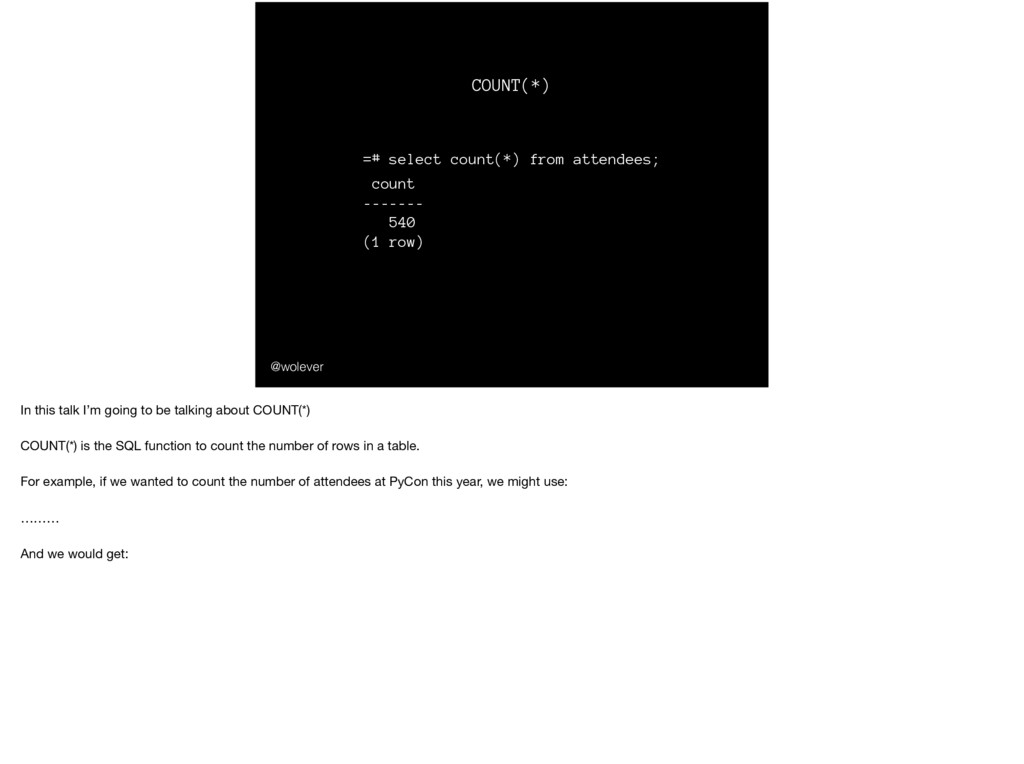
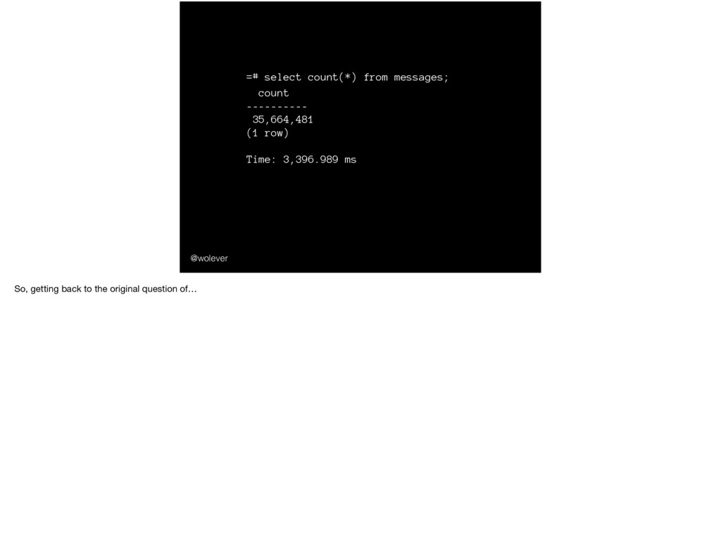
Time: 3,396.989 ms @wolever And one day at work I was trying to count the number of `messages` in our messages table: … … … Dang, that’s really slow. So I got curious: counting the number of rows in a table should be easy! What’s making it so dang slow?
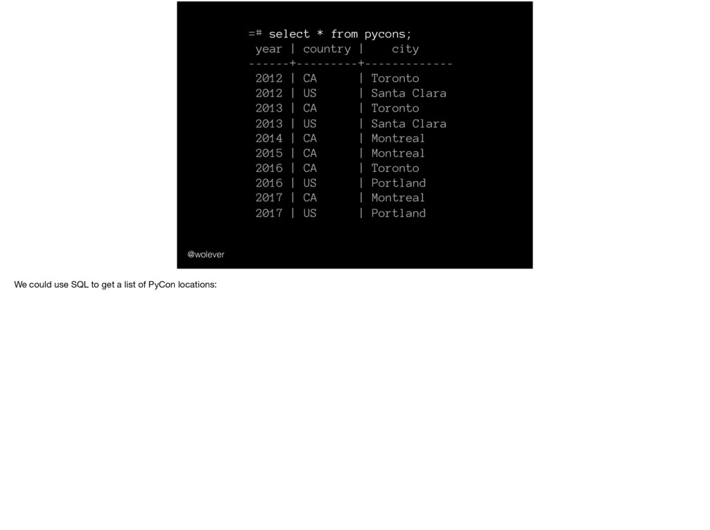
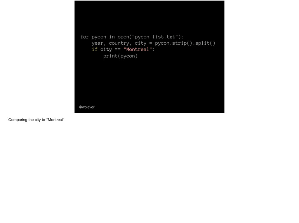
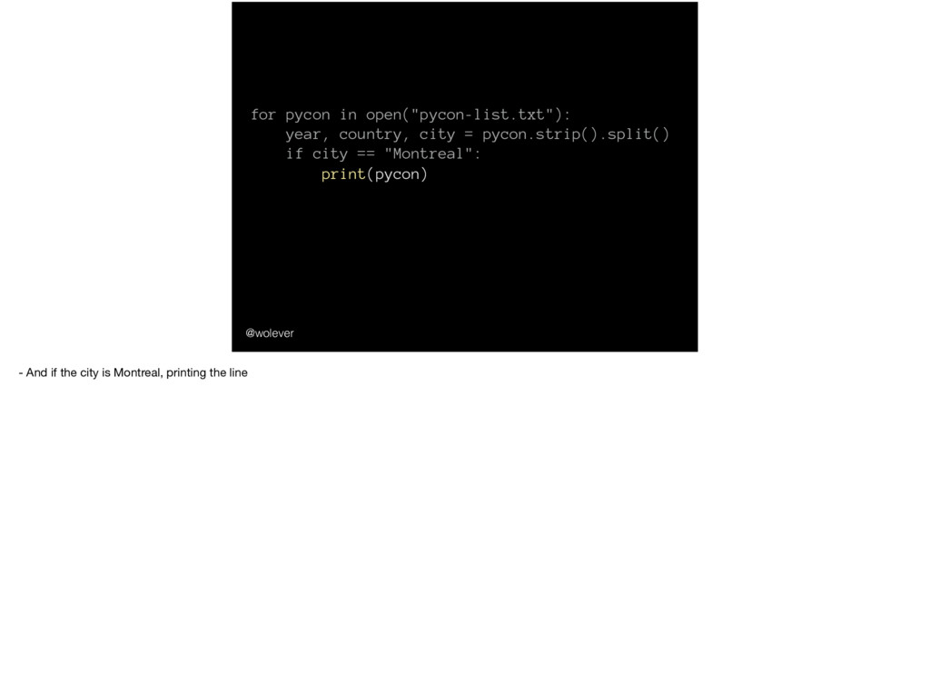
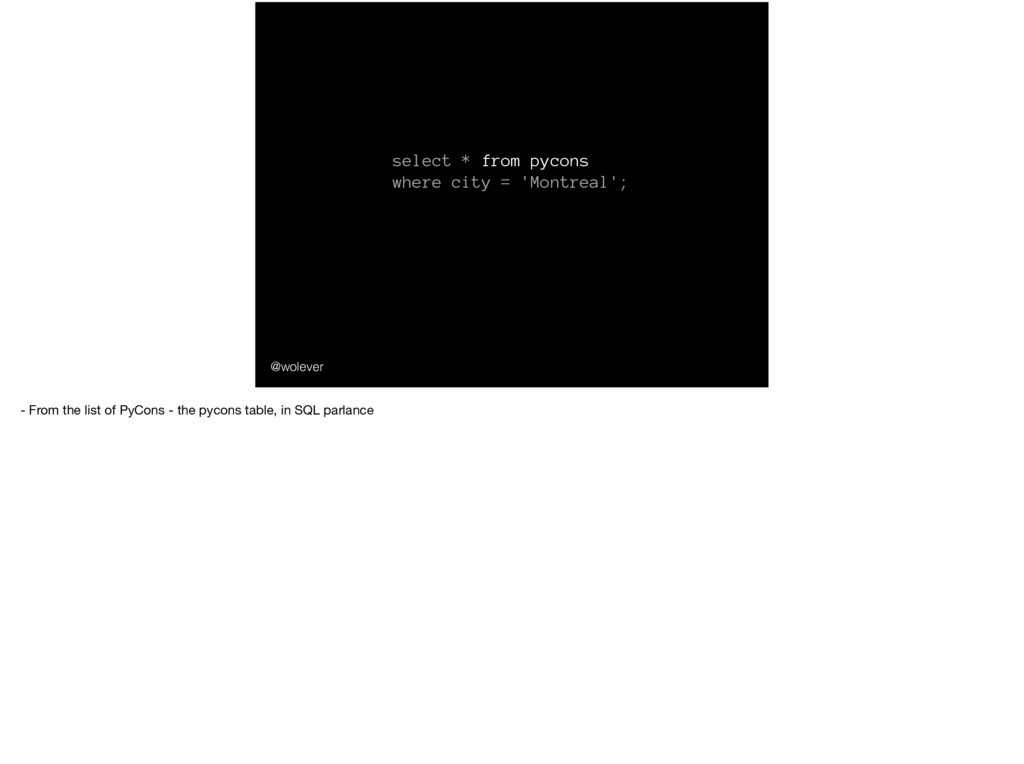
city ------+---------+------------- 2012 | CA | Toronto 2012 | US | Santa Clara 2013 | CA | Toronto 2013 | US | Santa Clara 2014 | CA | Montreal 2015 | CA | Montreal 2016 | CA | Toronto 2016 | US | Portland 2017 | CA | Montreal 2017 | US | Portland We could use SQL to get a list of PyCon locations:
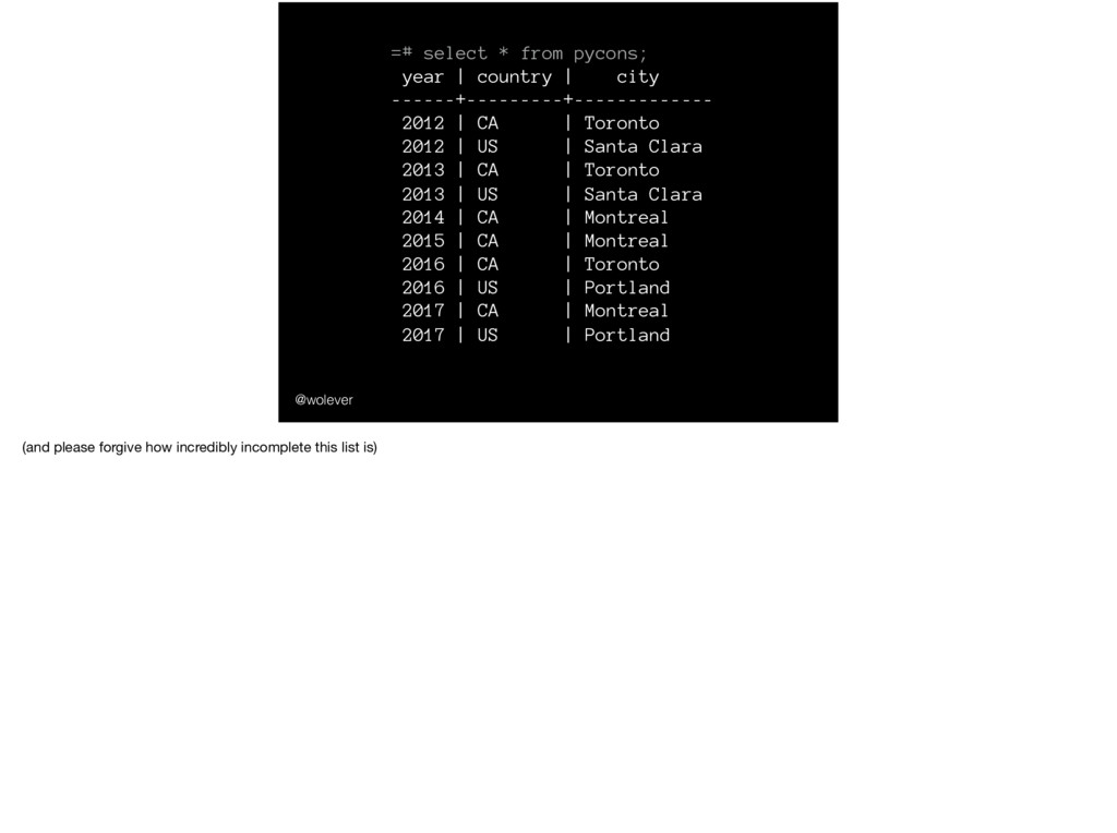
city ------+---------+------------- 2012 | CA | Toronto 2012 | US | Santa Clara 2013 | CA | Toronto 2013 | US | Santa Clara 2014 | CA | Montreal 2015 | CA | Montreal 2016 | CA | Toronto 2016 | US | Portland 2017 | CA | Montreal 2017 | US | Portland (and please forgive how incredibly incomplete this list is)
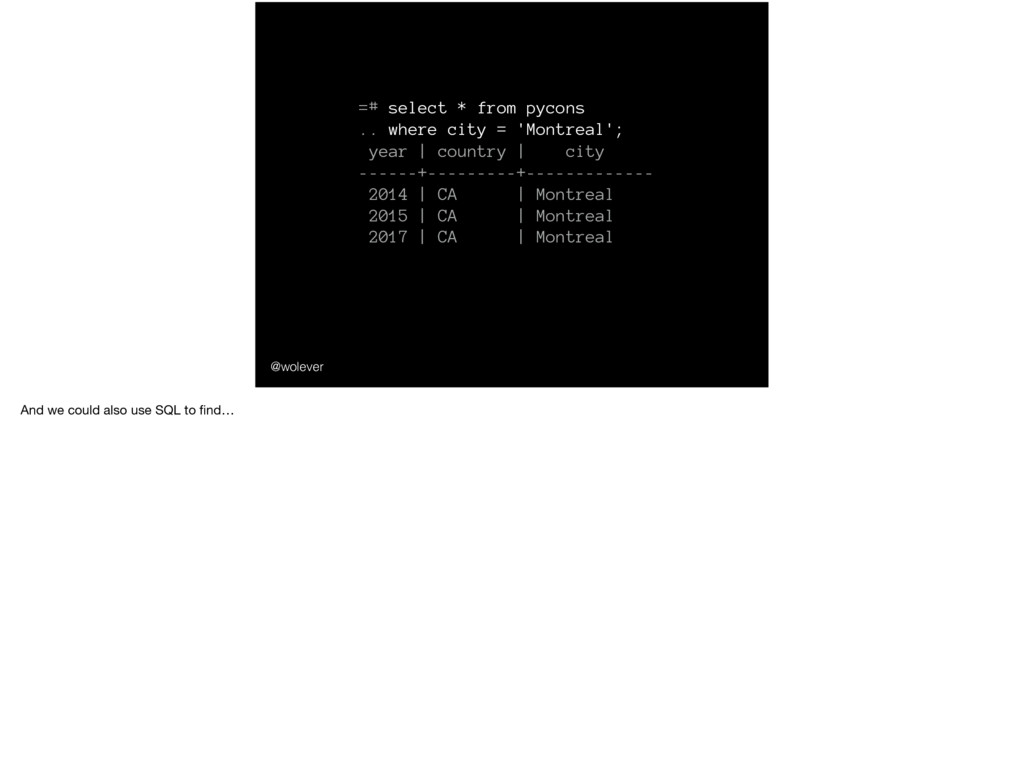
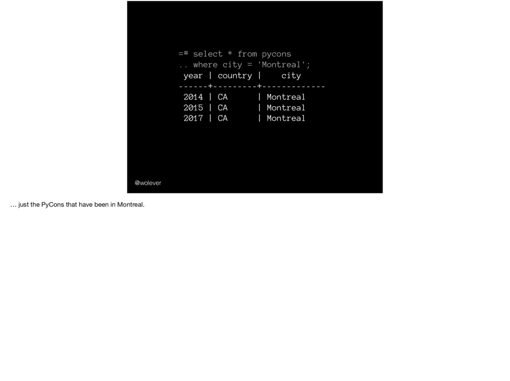
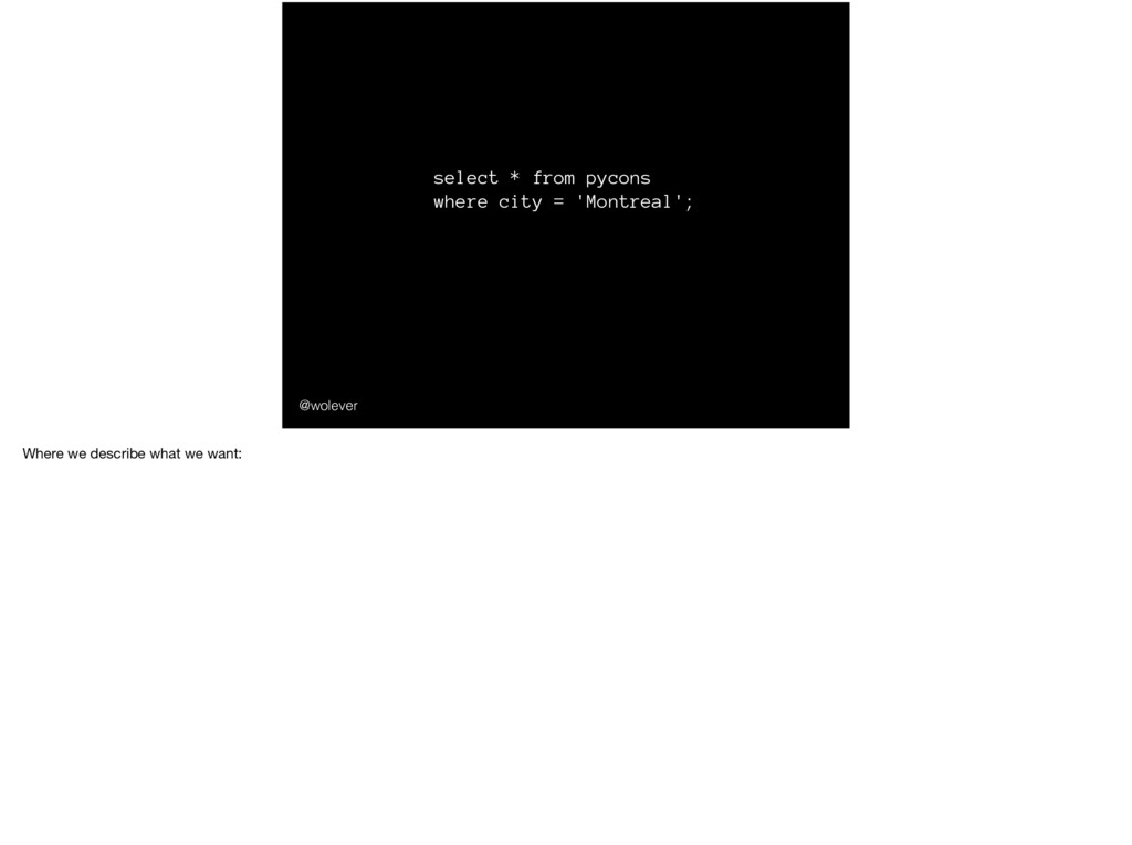
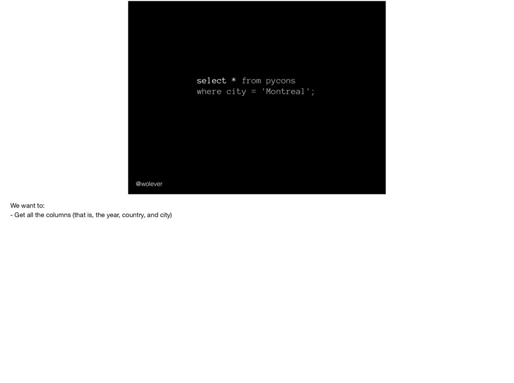
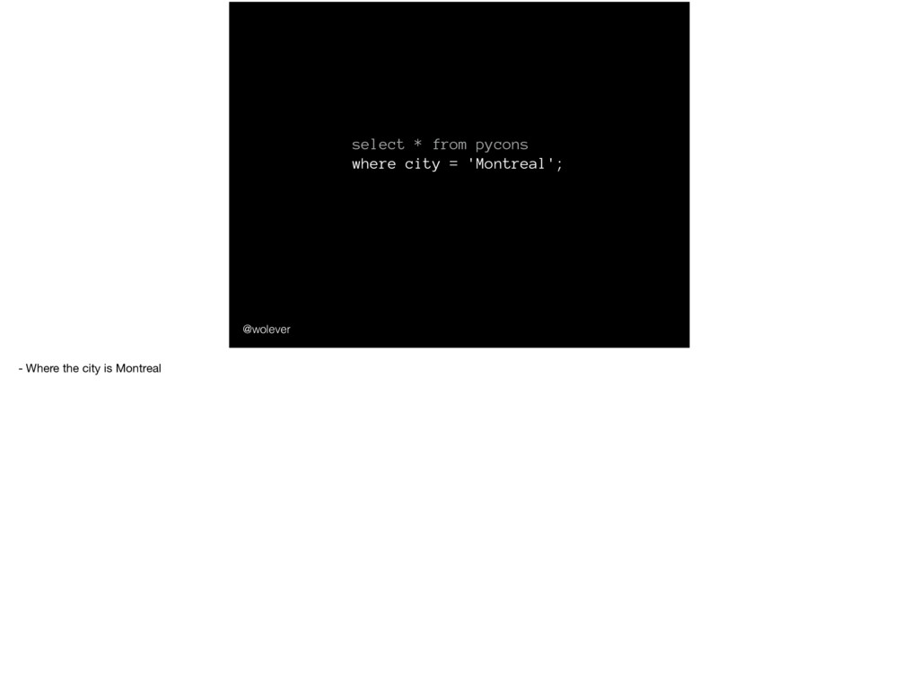
'Montreal'; year | country | city ------+---------+------------- 2014 | CA | Montreal 2015 | CA | Montreal 2017 | CA | Montreal And we could also use SQL to find…
'Montreal'; year | country | city ------+---------+------------- 2014 | CA | Montreal 2015 | CA | Montreal 2017 | CA | Montreal … just the PyCons that have been in Montreal.
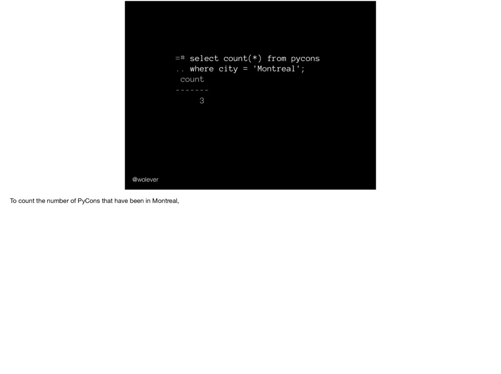
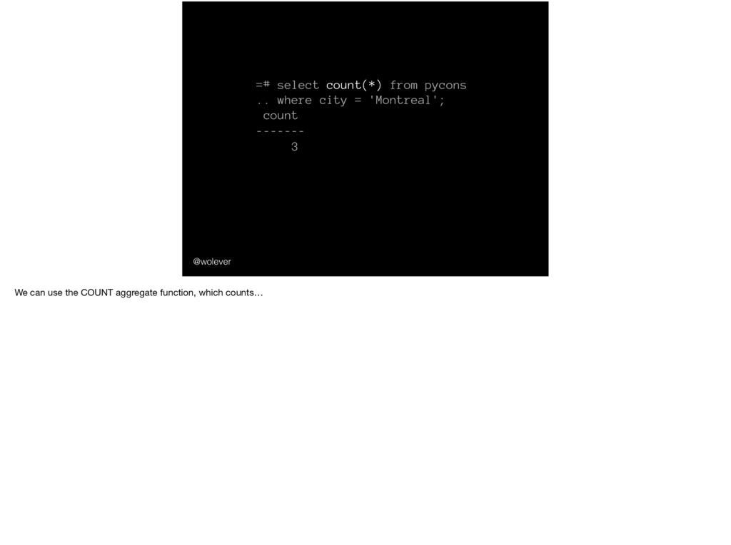
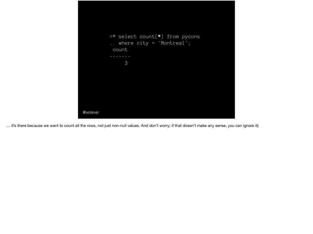
'Montreal'; count ------- 3 … it’s there because we want to count all the rows, not just non-null values. And don’t worry; if that doesn’t make any sense, you can ignore it).
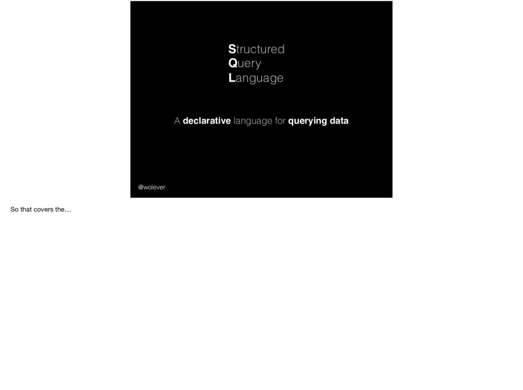
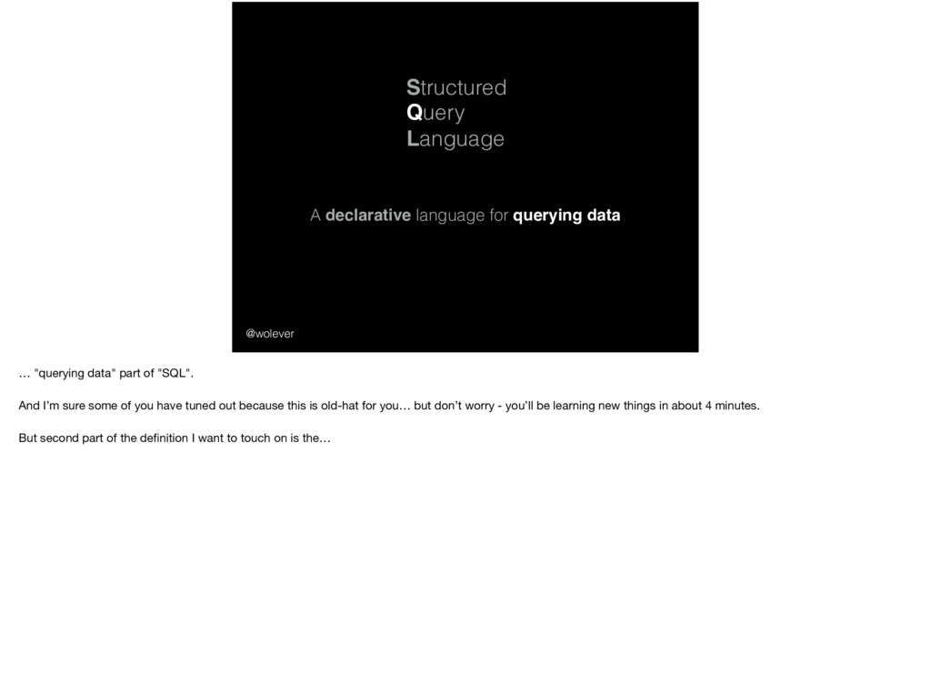
… "querying data" part of "SQL". And I’m sure some of you have tuned out because this is old-hat for you… but don’t worry - you’ll be learning new things in about 4 minutes. But second part of the definition I want to touch on is the…
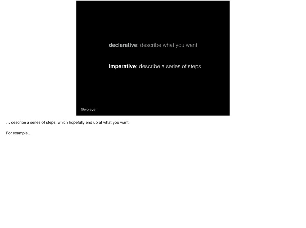
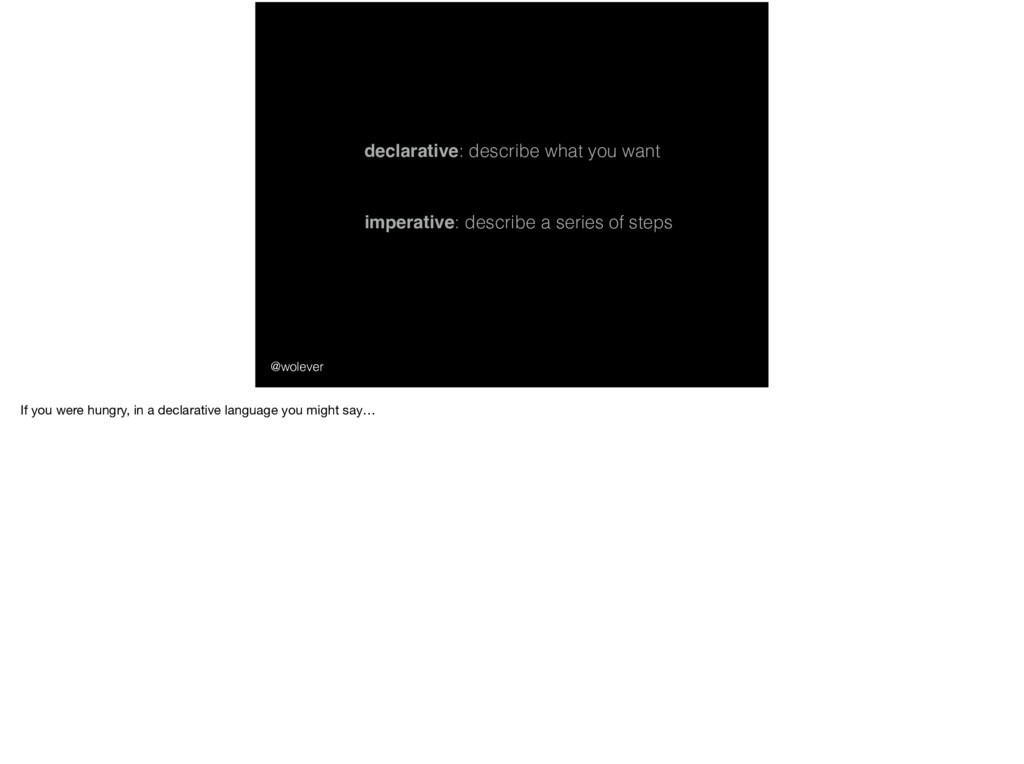
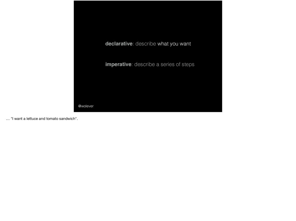
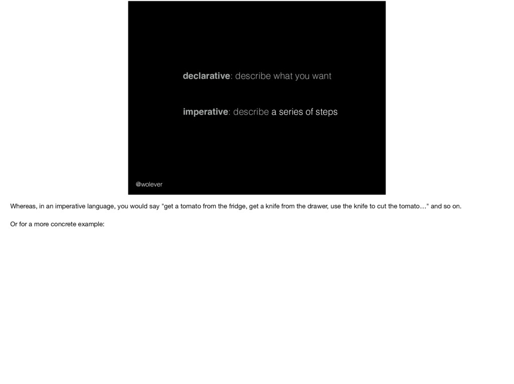
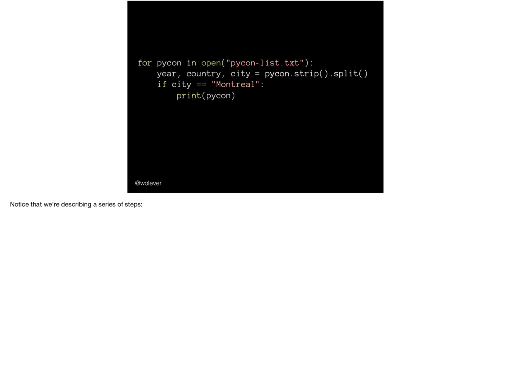
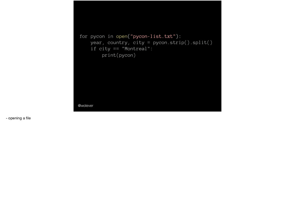
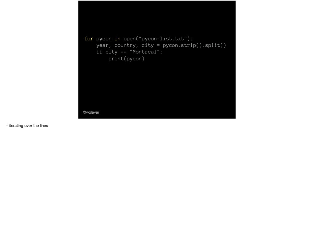
of steps Whereas, in an imperative language, you would say "get a tomato from the fridge, get a knife from the drawer, use the knife to cut the tomato…" and so on. Or for a more concrete example:
a big advantage of declarative languages is that they can be very powerful and descriptive; you tell the computer what you want, and it decides how to get that thing you want. But this comes at a cost: computers dumb, and sometimes they make bad decisions.
"under the hood" Now, with imperative languages, when the computer makes a bad decision or does something unexpected, it’s fairly straight forward to "peek under the hood" and see what’s going on; after all, you’ve described a series of small, granular steps.
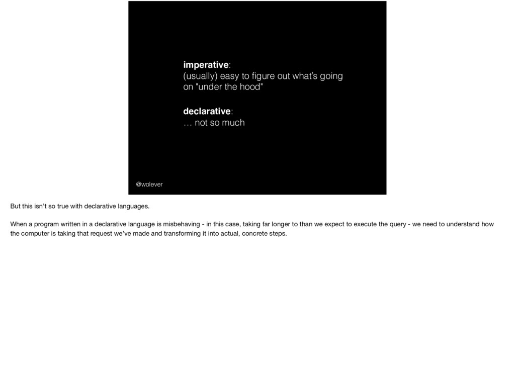
"under the hood" declarative: … not so much But this isn’t so true with declarative languages. When a program written in a declarative language is misbehaving - in this case, taking far longer to than we expect to execute the query - we need to understand how the computer is taking that request we’ve made and transforming it into actual, concrete steps.
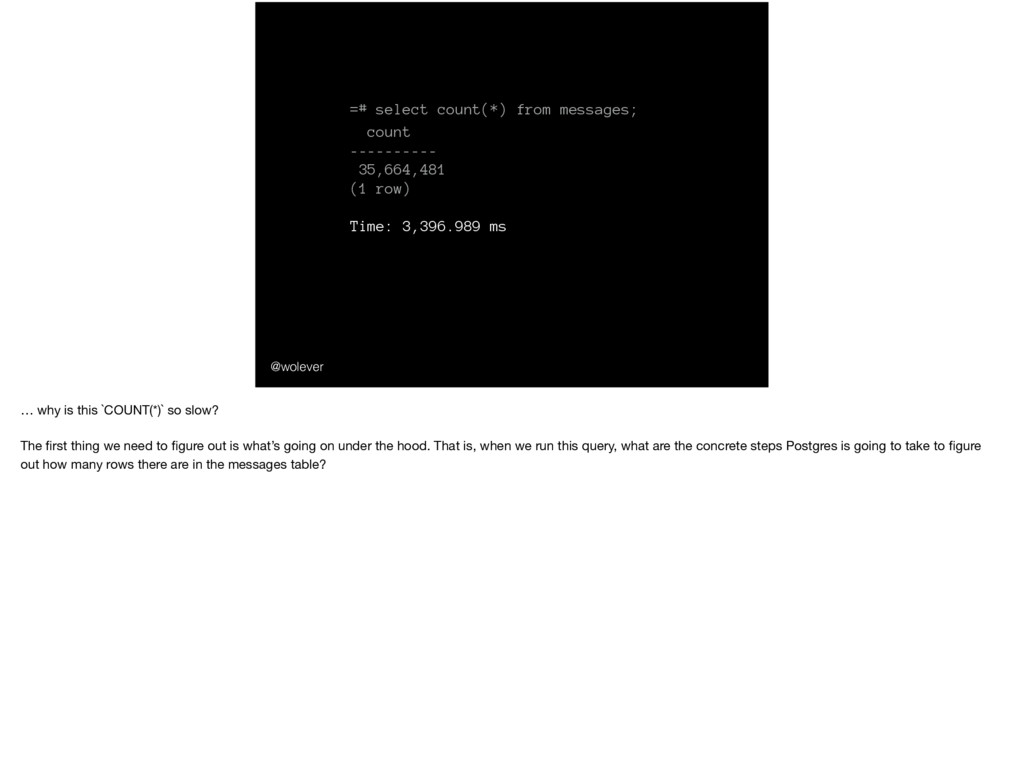
Time: 3,396.989 ms @wolever … why is this `COUNT(*)` so slow? The first thing we need to figure out is what’s going on under the hood. That is, when we run this query, what are the concrete steps Postgres is going to take to figure out how many rows there are in the messages table?
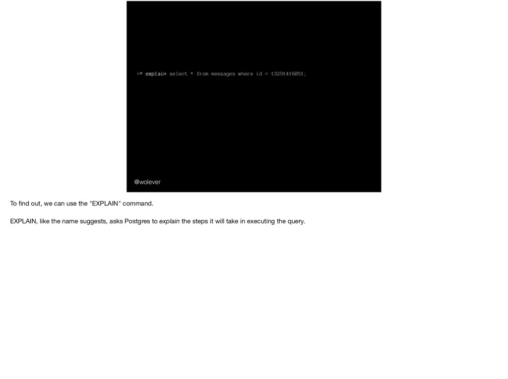
13291416051; QUERY PLAN ------------------------------------------------------------------------------ Index Scan using messages_id on messages (cost=0.56..8.79 rows=13 width=61) Index Cond: (id = '13291416051'::bigint) To find out, we can use the "EXPLAIN" command. EXPLAIN, like the name suggests, asks Postgres to explain the steps it will take in executing the query.
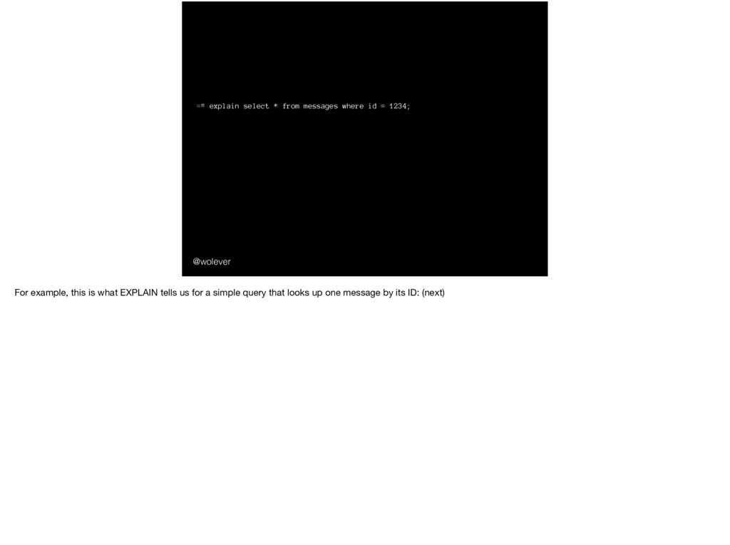
1234; QUERY PLAN ------------------------------------------------------------------------------ Index Scan using messages_id on messages (cost=0.56..8.79 rows=13 width=61) Index Cond: (id = '13291416051'::bigint) For example, this is what EXPLAIN tells us for a simple query that looks up one message by its ID: (next)
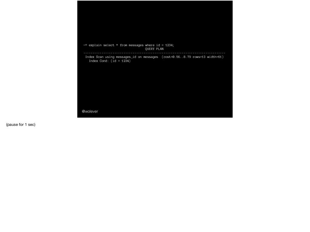
1234; QUERY PLAN ------------------------------------------------------------------------------ Index Scan using messages_id on messages (cost=0.56..8.79 rows=13 width=61) Index Cond: (id = 1234) (pause for 1 sec)
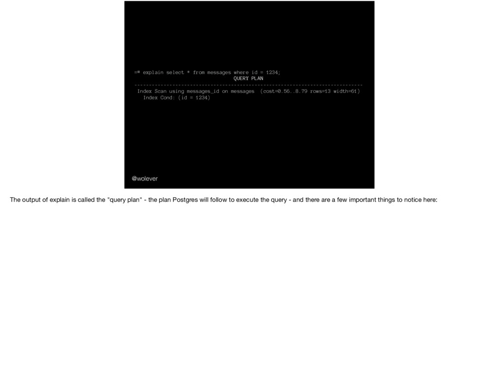
1234; QUERY PLAN ------------------------------------------------------------------------------ Index Scan using messages_id on messages (cost=0.56..8.79 rows=13 width=61) Index Cond: (id = 1234) The output of explain is called the "query plan" - the plan Postgres will follow to execute the query - and there are a few important things to notice here:
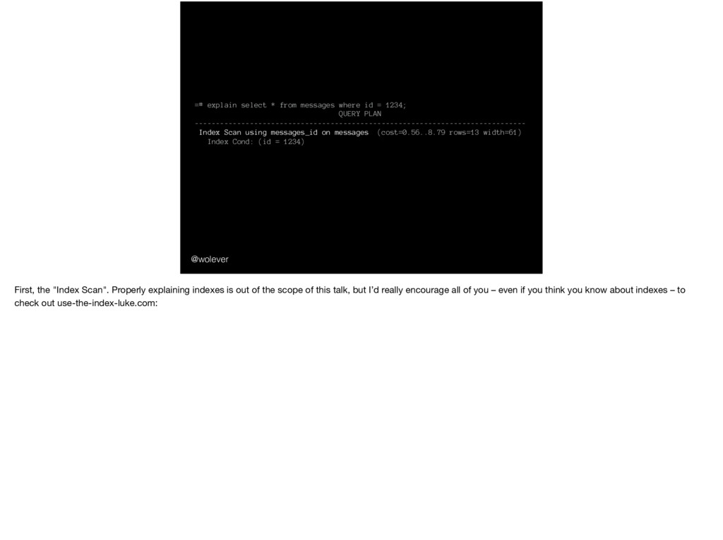
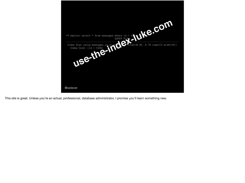
1234; QUERY PLAN ------------------------------------------------------------------------------ Index Scan using messages_id on messages (cost=0.56..8.79 rows=13 width=61) Index Cond: (id = 1234) First, the "Index Scan". Properly explaining indexes is out of the scope of this talk, but I’d really encourage all of you – even if you think you know about indexes – to check out use-the-index-luke.com:
1234; QUERY PLAN ------------------------------------------------------------------------------ Index Scan using messages_id on messages (cost=0.56..8.79 rows=13 width=61) Index Cond: (id = 1234) use-the-index-luke.com This site is great. Unless you’re an actual, professional, database administrator, I promise you’ll learn something new.
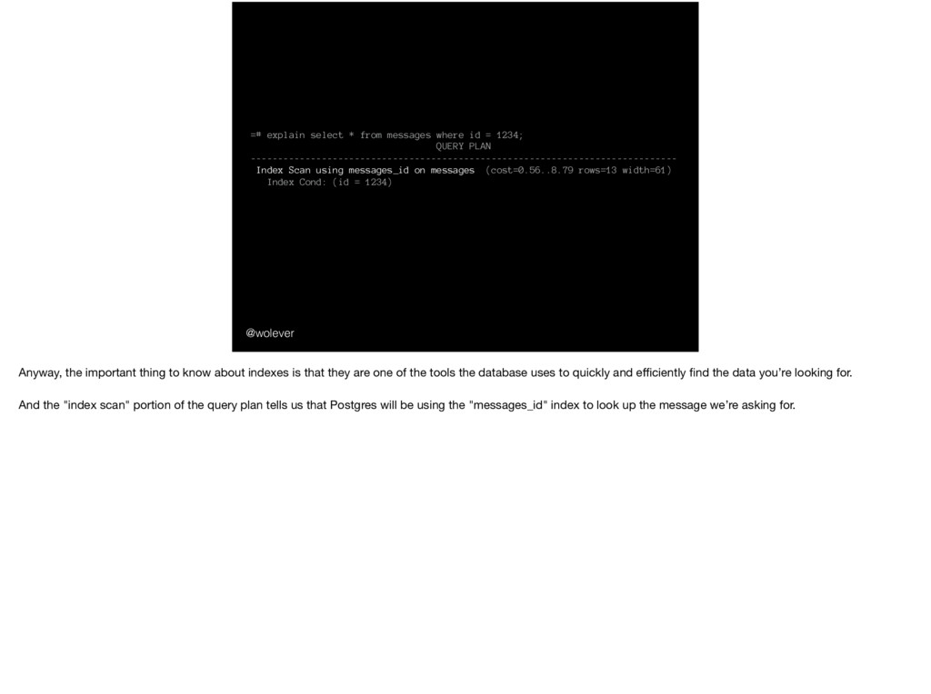
1234; QUERY PLAN ------------------------------------------------------------------------------ Index Scan using messages_id on messages (cost=0.56..8.79 rows=13 width=61) Index Cond: (id = 1234) Anyway, the important thing to know about indexes is that they are one of the tools the database uses to quickly and efficiently find the data you’re looking for. And the "index scan" portion of the query plan tells us that Postgres will be using the "messages_id" index to look up the message we’re asking for.
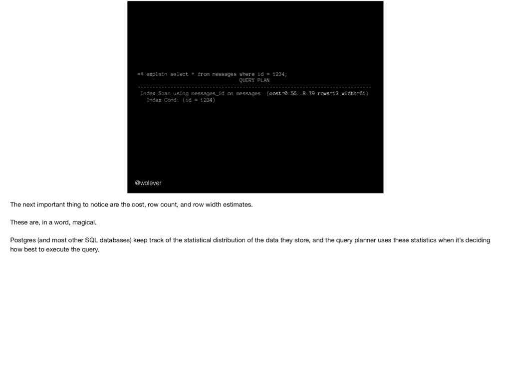
1234; QUERY PLAN ------------------------------------------------------------------------------ Index Scan using messages_id on messages (cost=0.56..8.79 rows=13 width=61) Index Cond: (id = 1234) The next important thing to notice are the cost, row count, and row width estimates. These are, in a word, magical. Postgres (and most other SQL databases) keep track of the statistical distribution of the data they store, and the query planner uses these statistics when it’s deciding how best to execute the query.
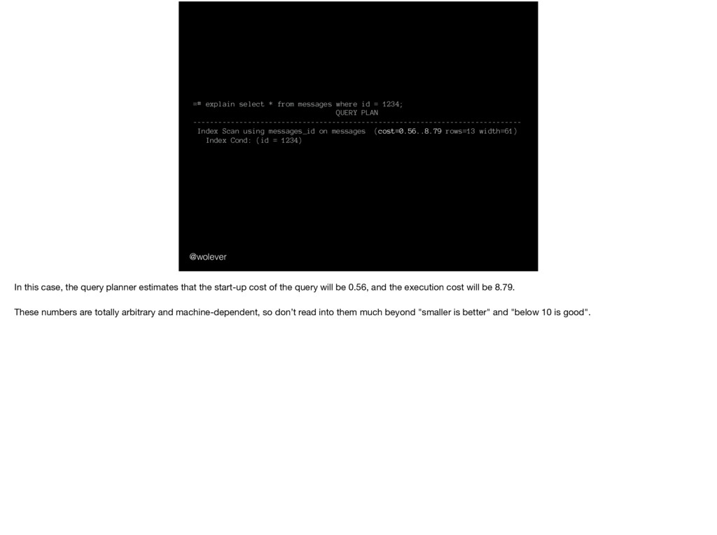
1234; QUERY PLAN ------------------------------------------------------------------------------ Index Scan using messages_id on messages (cost=0.56..8.79 rows=13 width=61) Index Cond: (id = 1234) In this case, the query planner estimates that the start-up cost of the query will be 0.56, and the execution cost will be 8.79. These numbers are totally arbitrary and machine-dependent, so don’t read into them much beyond "smaller is better" and "below 10 is good".
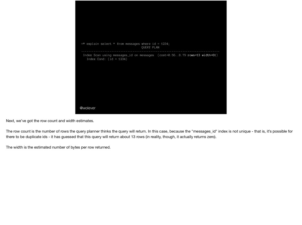
1234; QUERY PLAN ------------------------------------------------------------------------------ Index Scan using messages_id on messages (cost=0.56..8.79 rows=13 width=61) Index Cond: (id = 1234) Next, we’ve got the row count and width estimates. The row count is the number of rows the query planner thinks the query will return. In this case, because the "messages_id" index is not unique - that is, it’s possible for there to be duplicate ids - it has guessed that this query will return about 13 rows (in reality, though, it actually returns zero). The width is the estimated number of bytes per row returned.
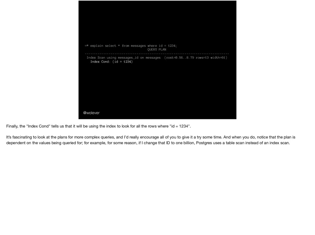
1234; QUERY PLAN ------------------------------------------------------------------------------ Index Scan using messages_id on messages (cost=0.56..8.79 rows=13 width=61) Index Cond: (id = 1234) Finally, the "Index Cond" tells us that it will be using the index to look for all the rows where "id = 1234". It’s fascinating to look at the plans for more complex queries, and I’d really encourage all of you to give it a try some time. And when you do, notice that the plan is dependent on the values being queried for; for example, for some reason, if I change that ID to one billion, Postgres uses a table scan instead of an index scan.
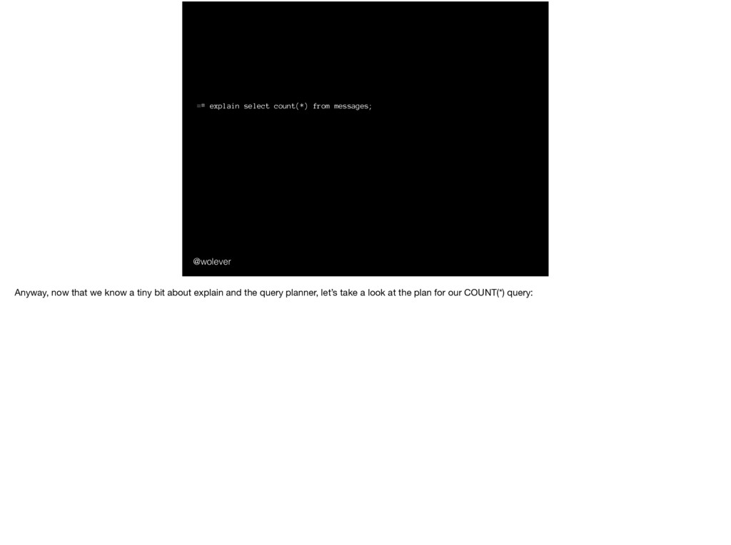
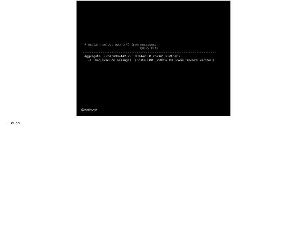
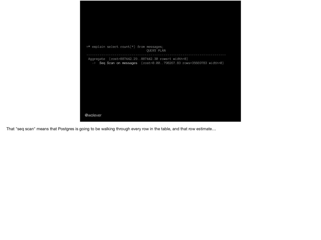
Aggregate (cost=887442.29..887442.30 rows=1 width=8) -> Seq Scan on messages (cost=0.00..798267.83 rows=35669783 width=0) Anyway, now that we know a tiny bit about explain and the query planner, let’s take a look at the plan for our COUNT(*) query:
Aggregate (cost=887442.29..887442.30 rows=1 width=8) -> Seq Scan on messages (cost=0.00..798267.83 rows=35669783 width=0) That "seq scan" means that Postgres is going to be walking through every row in the table, and that row estimate…
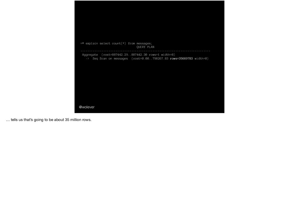
Aggregate (cost=887442.29..887442.30 rows=1 width=8) -> Seq Scan on messages (cost=0.00..798267.83 rows=35669783 width=0) … tells us that’s going to be about 35 million rows.
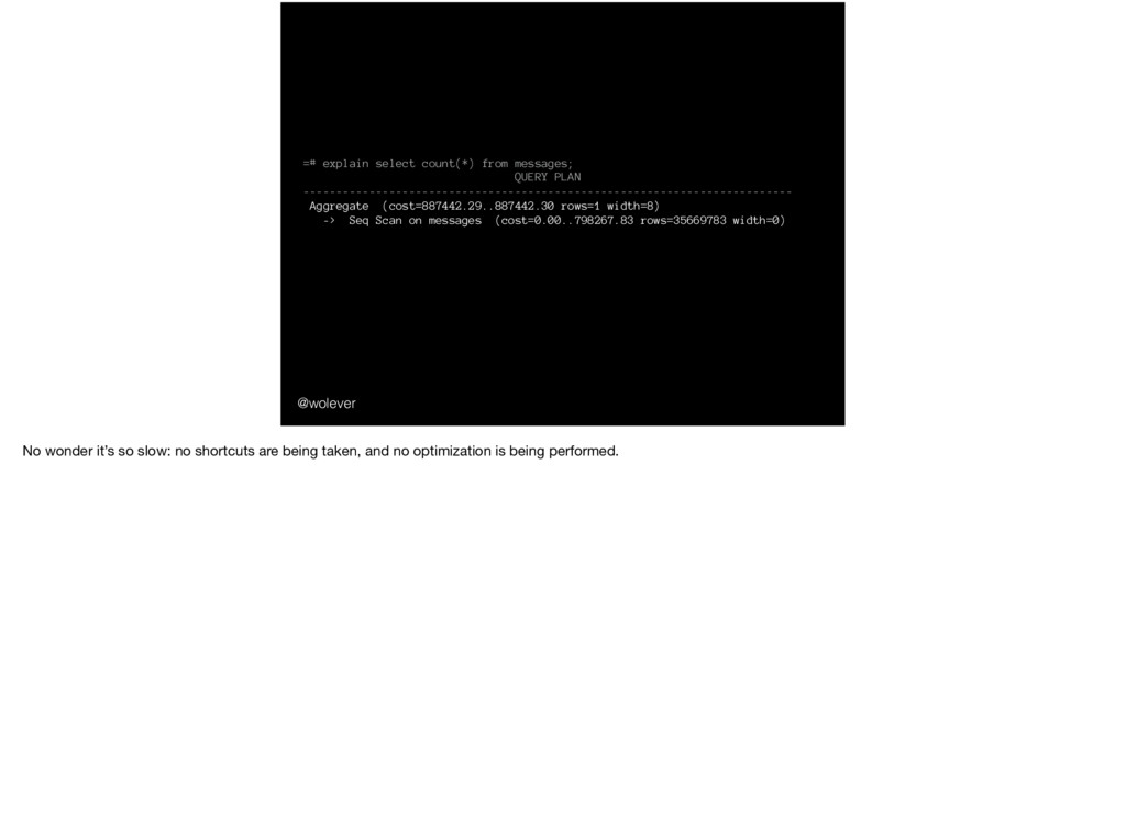
Aggregate (cost=887442.29..887442.30 rows=1 width=8) -> Seq Scan on messages (cost=0.00..798267.83 rows=35669783 width=0) No wonder it’s so slow: no shortcuts are being taken, and no optimization is being performed.
shouldn’t that be fast? And that seems pretty weird. After all, "counting all the things" is a pretty common operation, and databases are supposed to make common operations fast. Why shouldn’t that be fast?
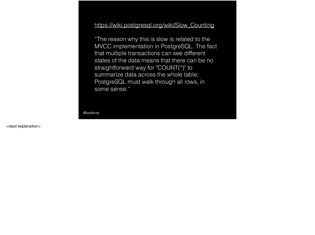
to the MVCC implementation in PostgreSQL. The fact that multiple transactions can see different states of the data means that there can be no straightforward way for "COUNT(*)" to summarize data across the whole table; PostgreSQL must walk through all rows, in some sense.” @wolever … the Postgres wiki page on "slow counting", which has this helpful explanation:
to the MVCC implementation in PostgreSQL. The fact that multiple transactions can see different states of the data means that there can be no straightforward way for "COUNT(*)" to summarize data across the whole table; PostgreSQL must walk through all rows, in some sense.” @wolever <read explanation>
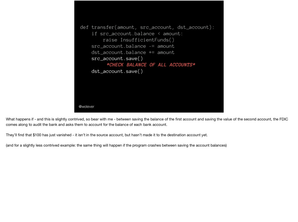
InsufficientFunds() src_account.balance -= amount dst_account.balance += amount src_account.save() *CHECK BALANCE OF ALL ACCOUNTS* dst_account.save() What happens if - and this is slightly contrived, so bear with me - between saving the balance of the first account and saving the value of the second account, the FDIC comes along to audit the bank and asks them to account for the balance of each bank account. They’ll find that $100 has just vanished - it isn’t in the source account, but hasn’t made it to the destination account yet. (and for a slightly less contrived example: the same thing will happen if the program crashes between saving the account balances)
(and all SQL databases) use to group a bunch of related queries together, making sure that other people querying the database can’t see intermediary results, and make sure the database doesn’t end up in an inconsistent state if something crashing in the middle of those queries. The best way to show how transactions work is with every speaker’s favourite thing…
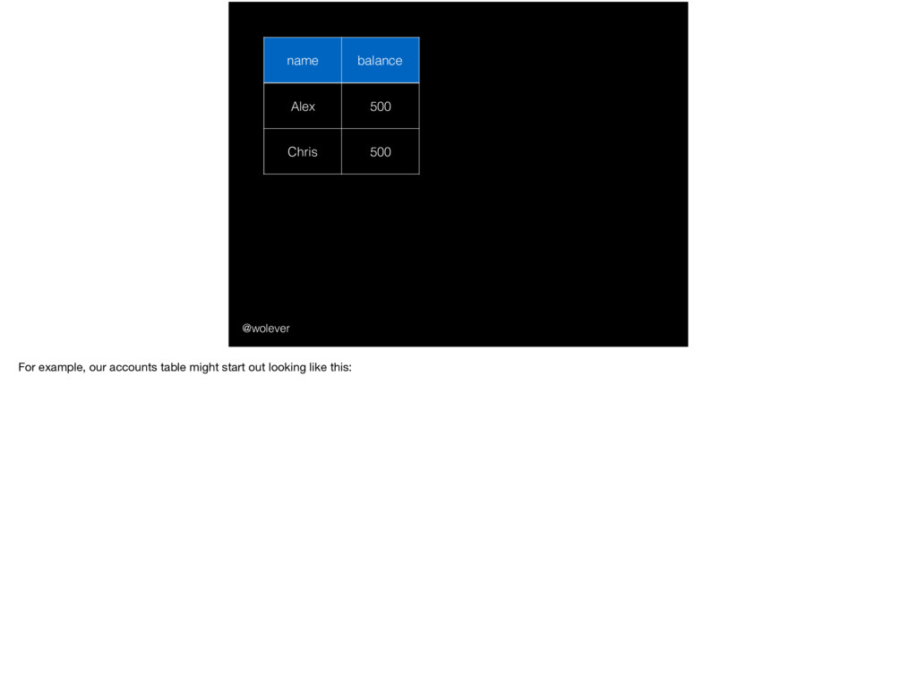
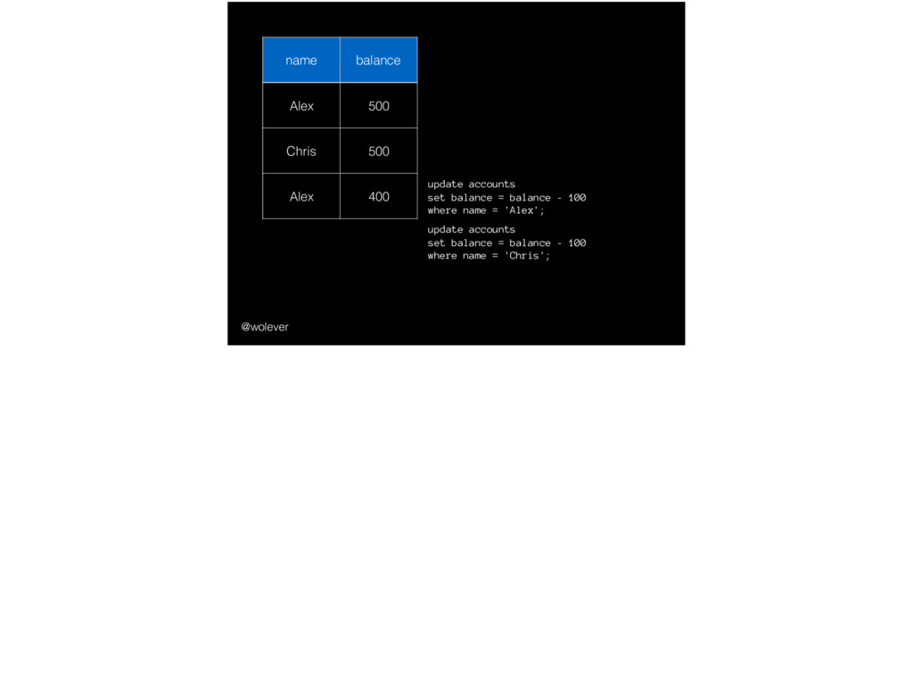
start with just two bank accounts: select * from accounts; - Next, from this other terminal, we’re going to transfer $100 from one to the other. We’ll start by creating a transaction with "begin": begin; - this tells postgres that the following commands only make sense to perform as a group. For example, when we deduct $100 from Alex’s account: update accounts set balance = balance - 100 where name = 'Alex'; - we should see the $100 deducted: select * from accounts; - but no one else should: select * from accounts; - once we’ve added that $100 into Chris’ account, though: update accounts set balance = balance + 100 where name = 'Chris';
To understand, we need to go one level deeper and find out exactly how transactions are implemented under the hood. How is it that Postgres can have one set of data for one transaction, and a different set of data for a different connection?
And I only used one transaction in this example… but it works just as well with 10, 100, or 1,000 transactions, each changing an arbitrarily large number of rows! How does that work?
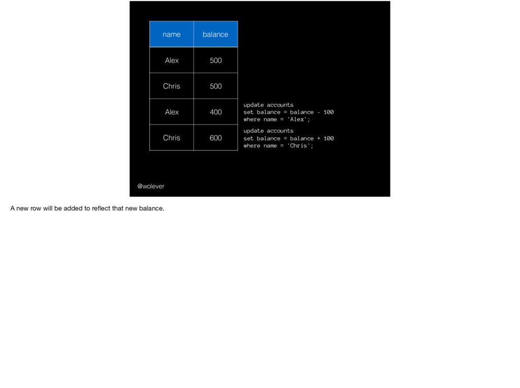
600 update accounts set balance = balance - 100 where name = 'Alex'; update accounts set balance = balance + 100 where name = 'Chris'; A new row will be added to reflect that new balance.
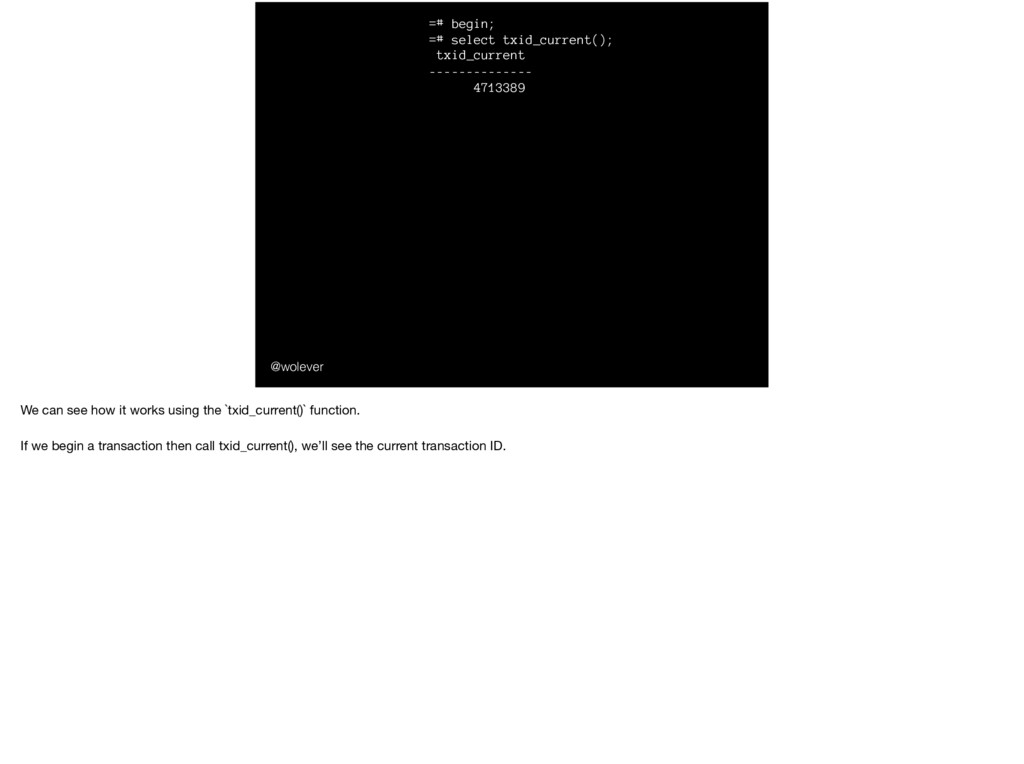
select txid_current(); txid_current -------------- 4713389 =# commit; =# begin; =# select txid_current(); txid_current -------------- 4713390 =# commit; =# select txid_current(); txid_current -------------- 4713391 We can see how it works using the `txid_current()` function. If we begin a transaction then call txid_current(), we’ll see the current transaction ID.
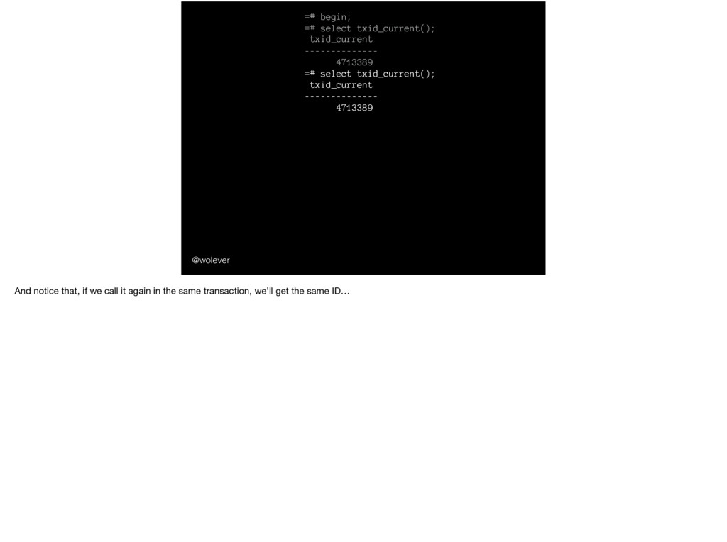
select txid_current(); txid_current -------------- 4713389 =# commit; =# begin; =# select txid_current(); txid_current -------------- 4713390 =# commit; =# select txid_current(); txid_current -------------- 4713391 And notice that, if we call it again in the same transaction, we’ll get the same ID…
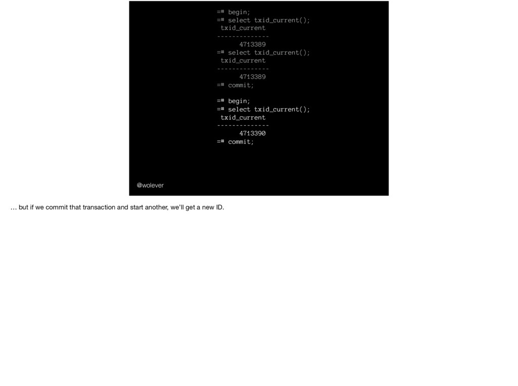
select txid_current(); txid_current -------------- 4713389 =# commit; =# begin; =# select txid_current(); txid_current -------------- 4713390 =# commit; =# select txid_current(); txid_current -------------- 4713391 … but if we commit that transaction and start another, we’ll get a new ID.
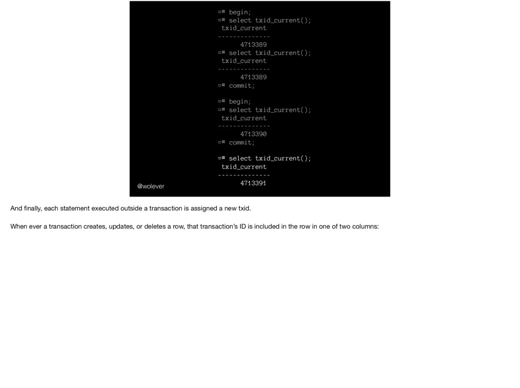
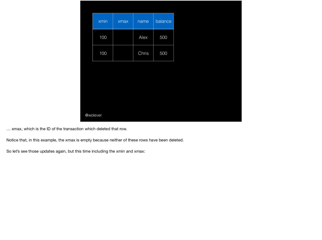
select txid_current(); txid_current -------------- 4713389 =# commit; =# begin; =# select txid_current(); txid_current -------------- 4713390 =# commit; =# select txid_current(); txid_current -------------- 4713391 And finally, each statement executed outside a transaction is assigned a new txid. When ever a transaction creates, updates, or deletes a row, that transaction’s ID is included in the row in one of two columns:
500 … xmax, which is the ID of the transaction which deleted that row. Notice that, in this example, the xmax is empty because neither of these rows have been deleted. So let’s see those updates again, but this time including the xmin and xmax:
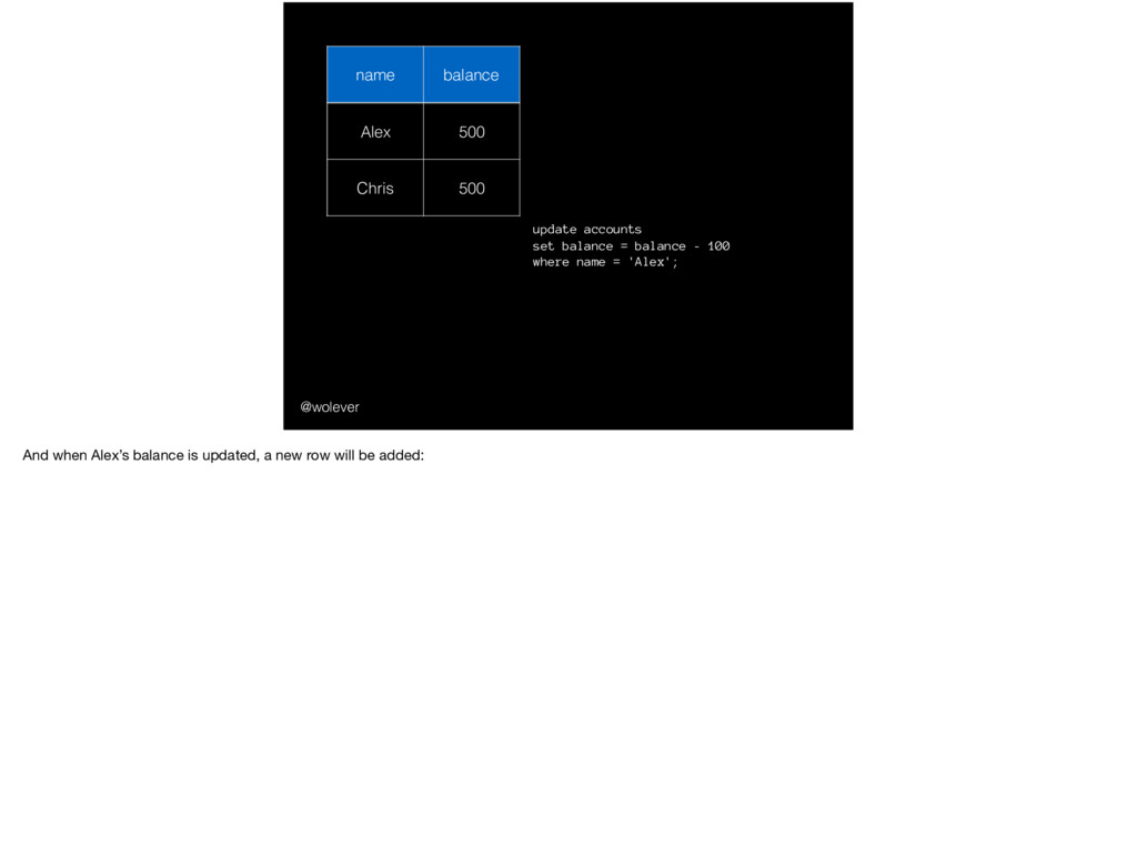
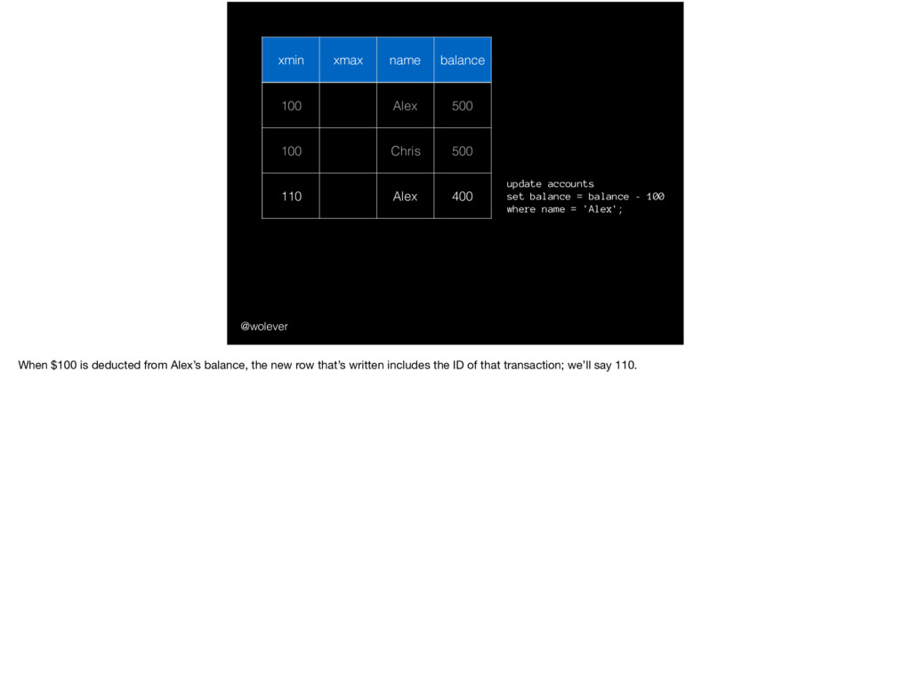
500 110 Alex 400 update accounts set balance = balance - 100 where name = 'Alex'; When $100 is deducted from Alex’s balance, the new row that’s written includes the ID of that transaction; we’ll say 110.
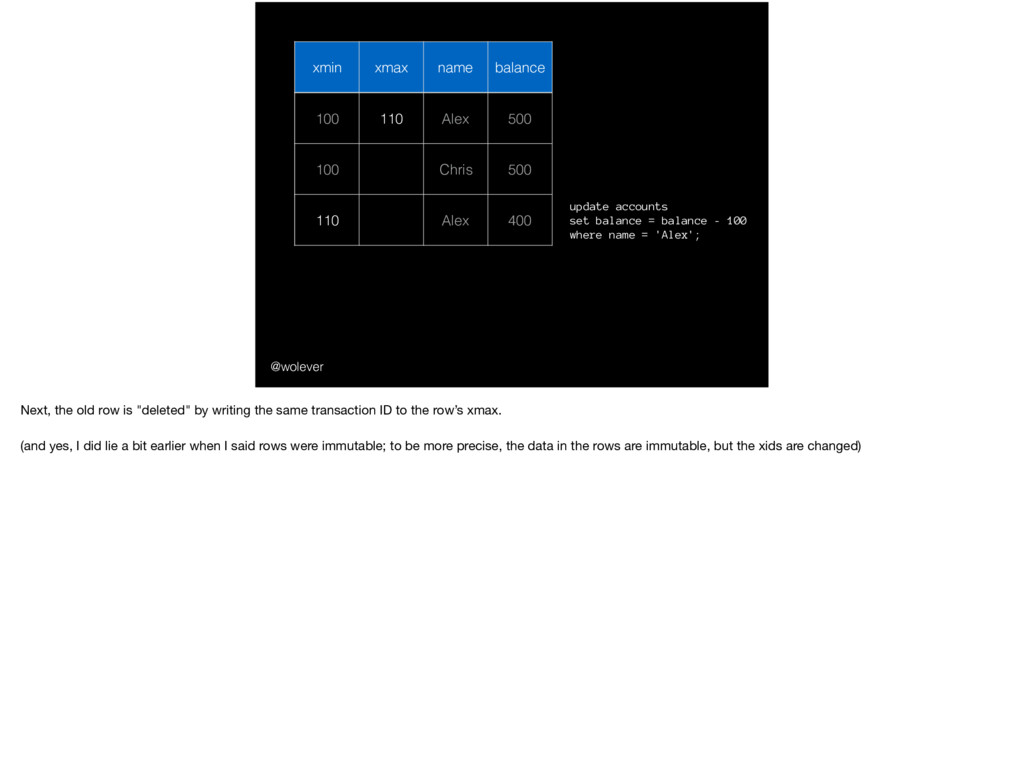
Chris 500 110 Alex 400 update accounts set balance = balance - 100 where name = 'Alex'; Next, the old row is "deleted" by writing the same transaction ID to the row’s xmax. (and yes, I did lie a bit earlier when I said rows were immutable; to be more precise, the data in the rows are immutable, but the xids are changed)
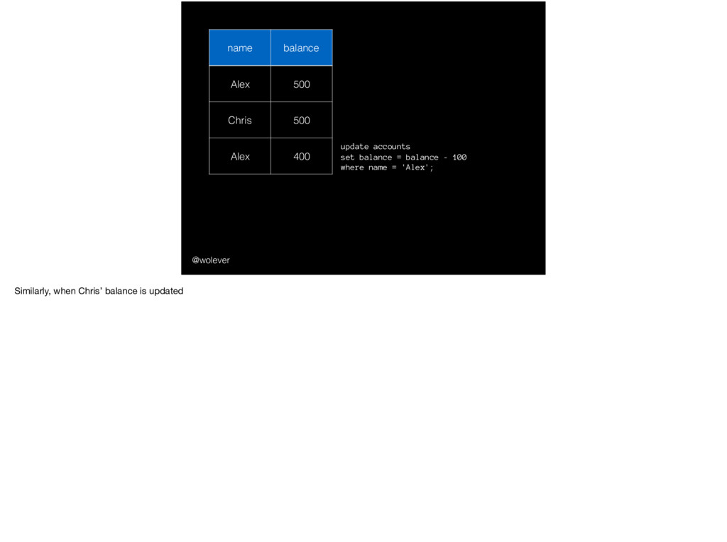
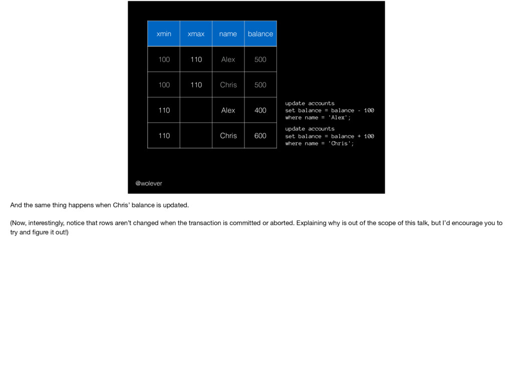
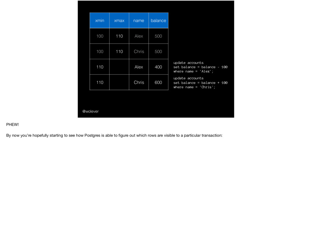
110 Chris 500 110 Alex 400 110 Chris 600 update accounts set balance = balance - 100 where name = 'Alex'; update accounts set balance = balance + 100 where name = 'Chris'; And the same thing happens when Chris’ balance is updated. (Now, interestingly, notice that rows aren’t changed when the transaction is committed or aborted. Explaining why is out of the scope of this talk, but I’d encourage you to try and figure it out!)
110 Chris 500 110 Alex 400 110 Chris 600 update accounts set balance = balance - 100 where name = 'Alex'; update accounts set balance = balance + 100 where name = 'Chris'; PHEW! By now you’re hopefully starting to see how Postgres is able to figure out which rows are visible to a particular transaction:
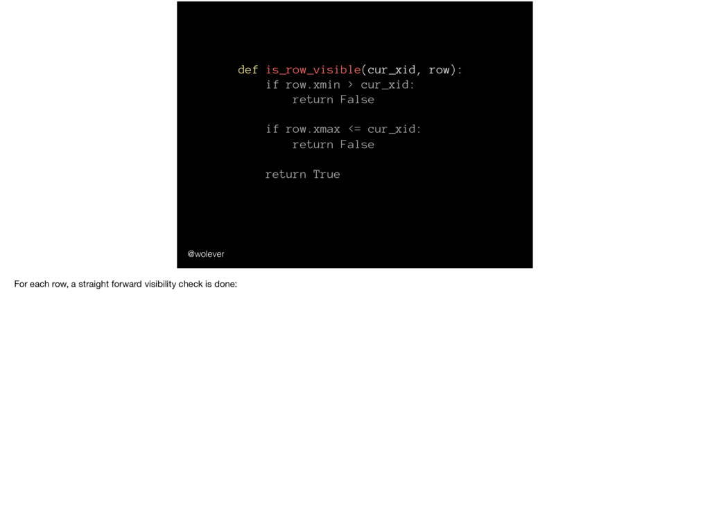
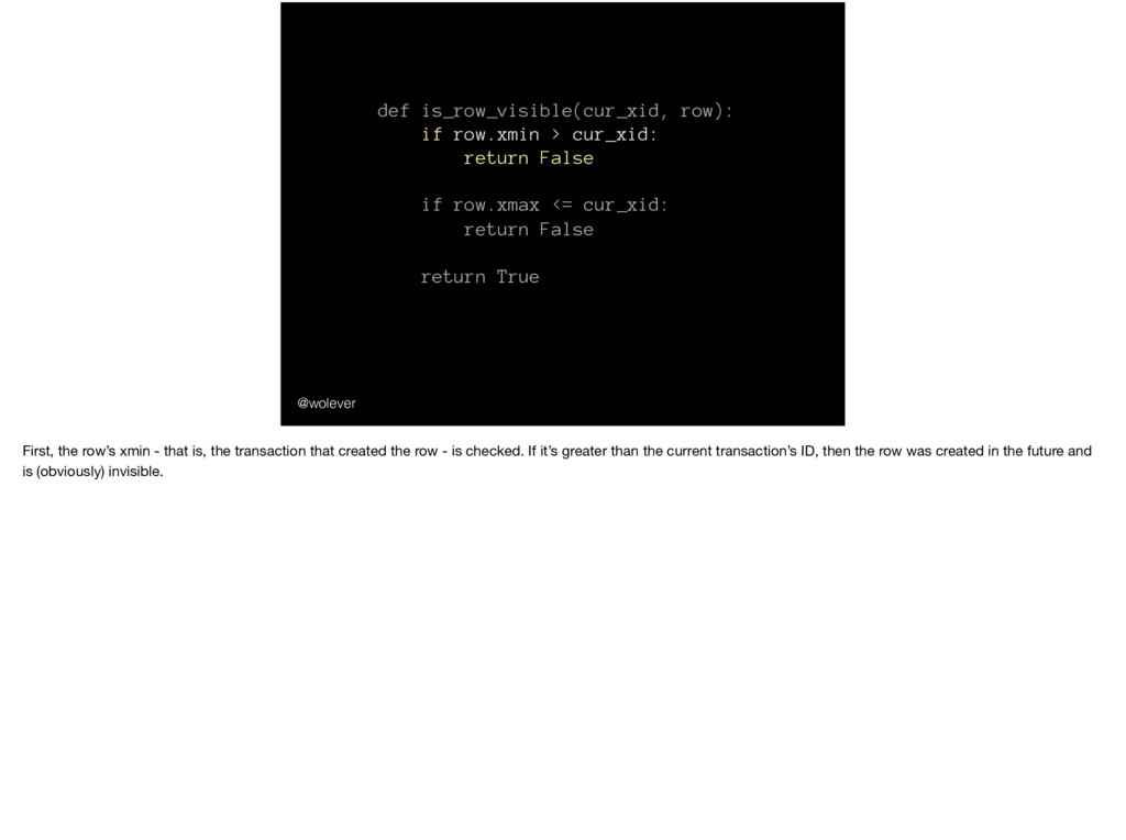
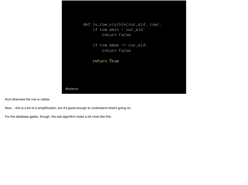
row.xmax <= cur_xid: return False return True @wolever First, the row’s xmin - that is, the transaction that created the row - is checked. If it’s greater than the current transaction’s ID, then the row was created in the future and is (obviously) invisible.
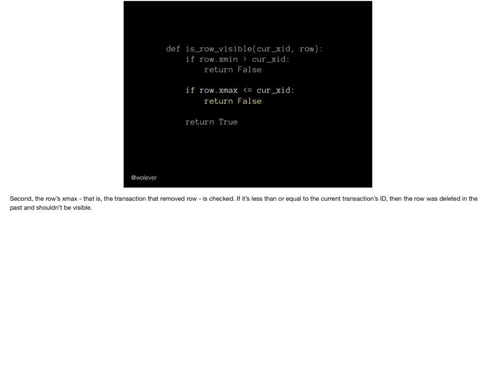
row.xmax <= cur_xid: return False return True @wolever Second, the row’s xmax - that is, the transaction that removed row - is checked. If it’s less than or equal to the current transaction’s ID, then the row was deleted in the past and shouldn’t be visible.
row.xmax <= cur_xid: return False return True @wolever And otherwise the row is visible. Now… this is a bit of a simplification, but it’s good enough to understand what’s going on. For the database geeks, though, the real algorithm looks a bit more like this:
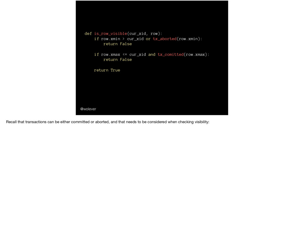
False if row.xmax <= cur_xid and tx_comitted(row.xmax): return False return True @wolever Recall that transactions can be either committed or aborted, and that needs to be considered when checking visibility:
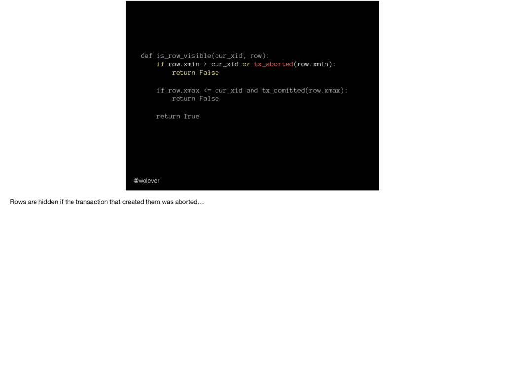
False if row.xmax <= cur_xid and tx_comitted(row.xmax): return False return True @wolever Rows are hidden if the transaction that created them was aborted…
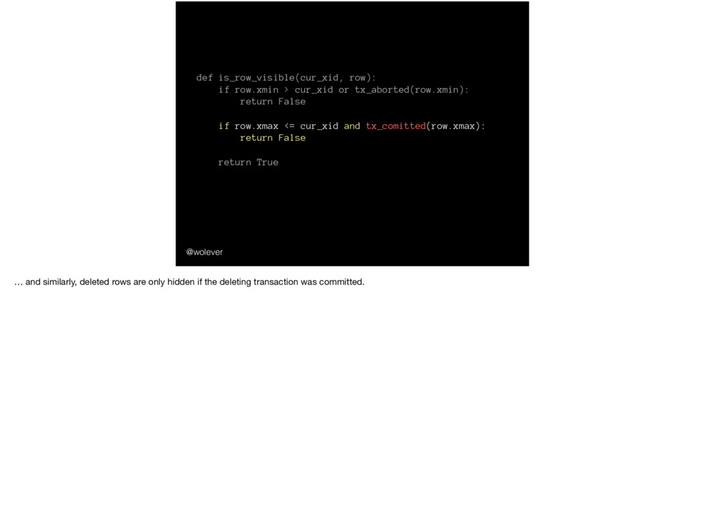
False if row.xmax <= cur_xid and tx_comitted(row.xmax): return False return True @wolever … and similarly, deleted rows are only hidden if the deleting transaction was committed.
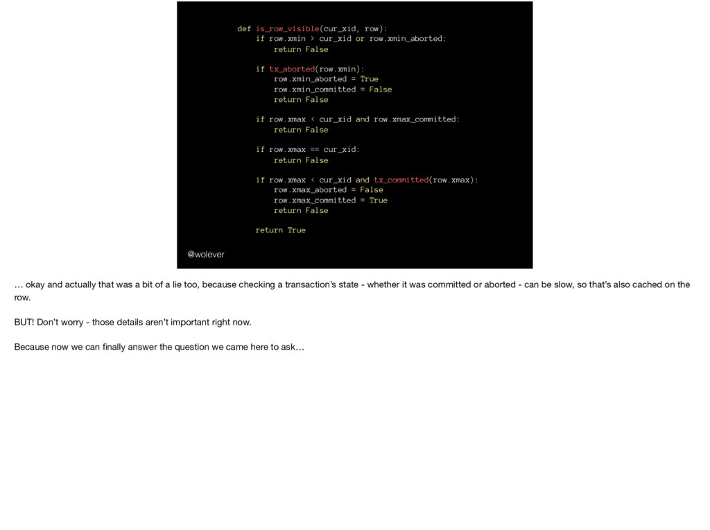
False if tx_aborted(row.xmin): row.xmin_aborted = True row.xmin_committed = False return False if row.xmax < cur_xid and row.xmax_committed: return False if row.xmax == cur_xid: return False if row.xmax < cur_xid and tx_committed(row.xmax): row.xmax_aborted = False row.xmax_committed = True return False return True @wolever … okay and actually that was a bit of a lie too, because checking a transaction’s state - whether it was committed or aborted - can be slow, so that’s also cached on the row. BUT! Don’t worry - those details aren’t important right now. Because now we can finally answer the question we came here to ask…
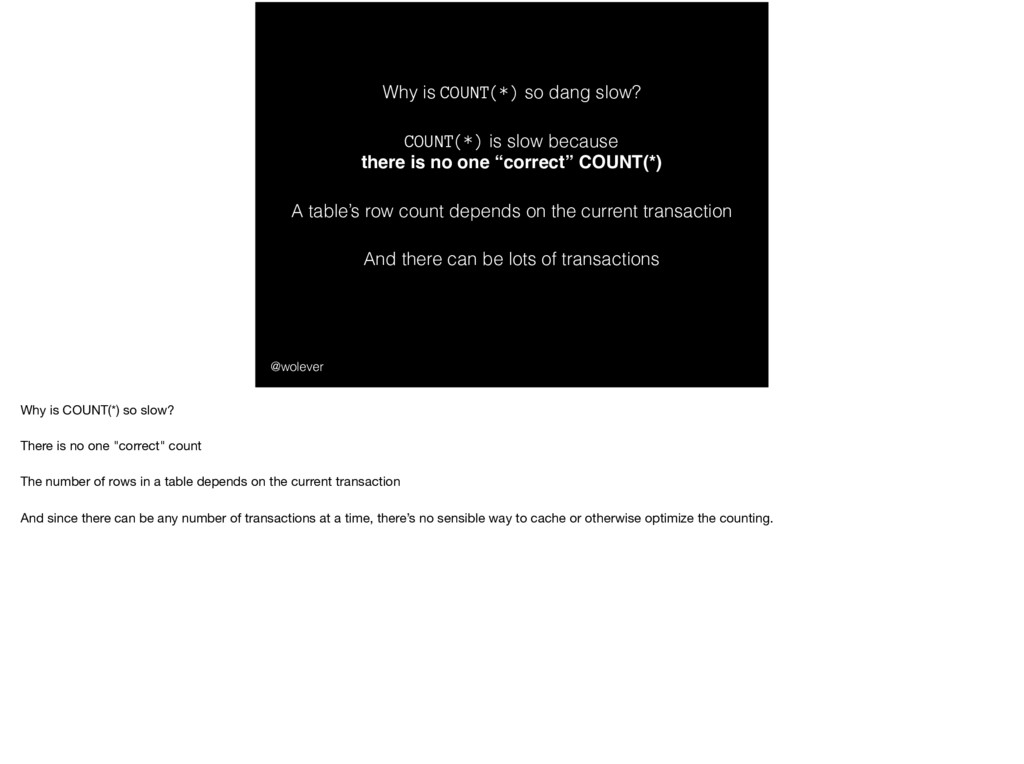
A table’s row count depends on the current transaction @wolever Why is COUNT(*) so dang slow? And there can be lots of transactions Why is COUNT(*) so slow? There is no one "correct" count The number of rows in a table depends on the current transaction And since there can be any number of transactions at a time, there’s no sensible way to cache or otherwise optimize the counting.
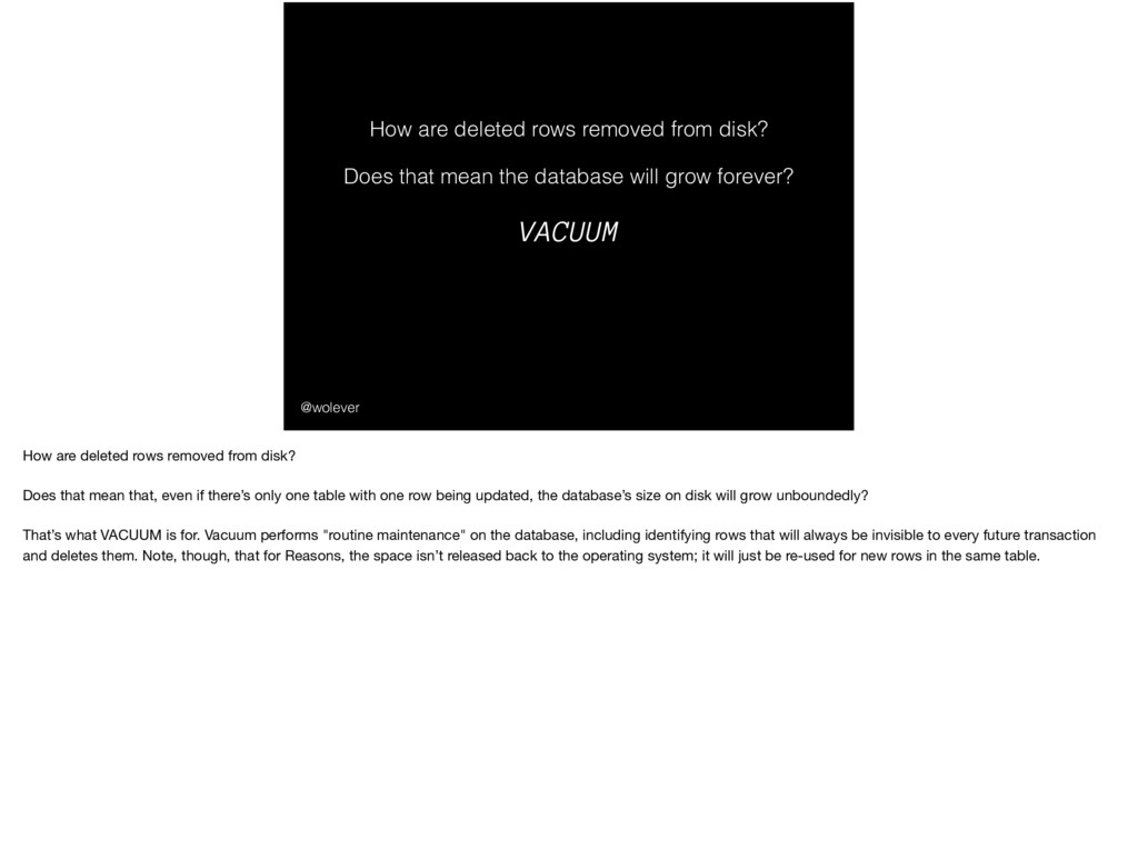
that mean the database will grow forever? How are deleted rows removed from disk? Does that mean that, even if there’s only one table with one row being updated, the database’s size on disk will grow unboundedly? That’s what VACUUM is for. Vacuum performs "routine maintenance" on the database, including identifying rows that will always be invisible to every future transaction and deletes them. Note, though, that for Reasons, the space isn’t released back to the operating system; it will just be re-used for new rows in the same table.
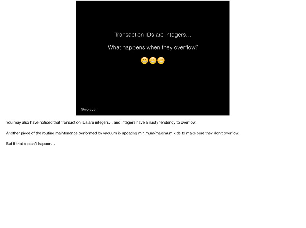
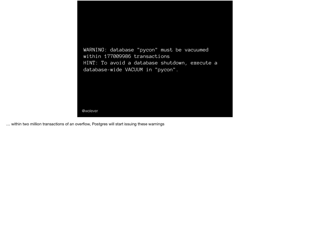
You may also have noticed that transaction IDs are integers… and integers have a nasty tendency to overflow. Another piece of the routine maintenance performed by vacuum is updating minimum/maximum xids to make sure they don’t overflow. But if that doesn’t happen…
To avoid a database shutdown, execute a database-wide VACUUM in "pycon". @wolever … within two million transactions of an overflow, Postgres will start issuing these warnings
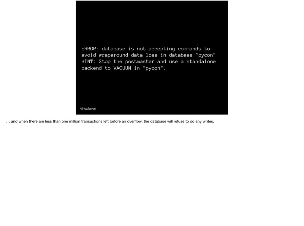
loss in database "pycon" HINT: Stop the postmaster and use a standalone backend to VACUUM in "pycon". @wolever … and when there are less than one million transactions left before an overflow, the database will refuse to do any writes.
hiring! My company, Akindi, builds a product that lets teachers print Scantron-style bubble sheets from any printer, scan them from any scanner, and get all the results online. We are - and this isn’t bragging, it’s an objective fact - the best on the market at what we do… and that’s mostly because we’re the only product in our market built after the year 2000. So if you’d enjoy working on software that makes teacher’s lives less terrible, come say hi! I’d love to chat with you!
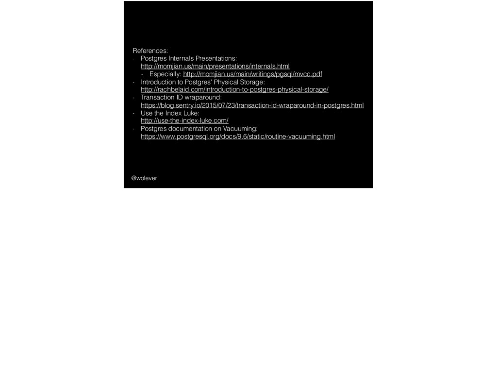
Introduction to Postgres' Physical Storage: http://rachbelaid.com/introduction-to-postgres-physical-storage/ - Transaction ID wraparound: https://blog.sentry.io/2015/07/23/transaction-id-wraparound-in-postgres.html - Use the Index Luke: http://use-the-index-luke.com/ - Postgres documentation on Vacuuming: https://www.postgresql.org/docs/9.6/static/routine-vacuuming.html @wolever
![David Wolever @wolever Work with me: [email protected] https://akindi.com/pages/jobs Also, I’m](https://files.speakerdeck.com/presentations/35a974babca444efb7cd96814626b048/slide_123.jpg)