[CS Foundation] Algorithm - 25 - All-Pairs Shortest Paths

Transcript

1. Chapter 25 All-Pairs Shortest Paths Sun-Yuan Hsieh 謝孫源 教授 成功大學資訊工程學系
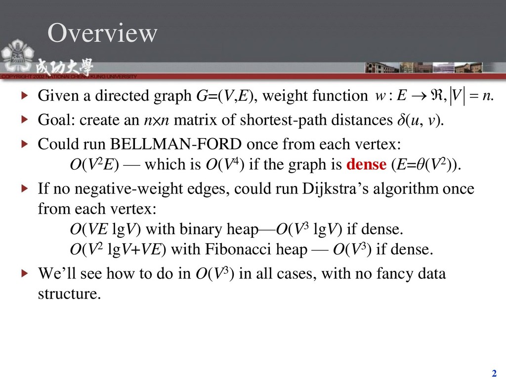
2. 2 Overview Given a directed graph G=(V,E), weight function Goal: create an n×n matrix of shortest-path distances δ(u, v). Could run BELLMAN-FORD once from each vertex: O(V2E) — which is O(V4) if the graph is dense (E=θ(V2)). If no negative-weight edges, could run Dijkstra’s algorithm once from each vertex: O(VE lgV) with binary heap—O(V3 lgV) if dense. O(V2 lgV+VE) with Fibonacci heap — O(V3) if dense. We’ll see how to do in O(V3) in all cases, with no fancy data structure. . , : n V E w   
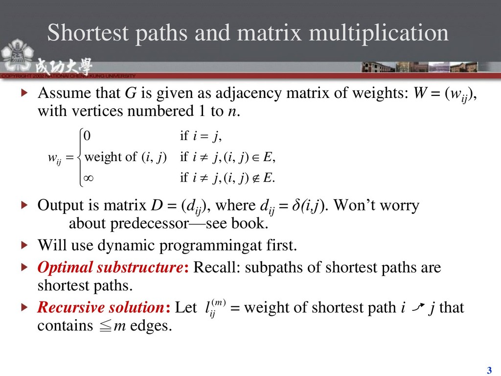
3. 3 Shortest paths and matrix multiplication Assume that G is given as adjacency matrix of weights: W = (wij ), with vertices numbered 1 to n. Output is matrix D = (dij ), where dij = δ(i,j). Won’t worry about predecessor—see book. Will use dynamic programmingat first. Optimal substructure: Recall: subpaths of shortest paths are shortest paths. Recursive solution: Let = weight of shortest path i j that contains ≦m edges.             . ) , ( , if , ) , ( , if ) , ( of weight , if 0 E j i j i E j i j i j i j i w ij ) (m ij l
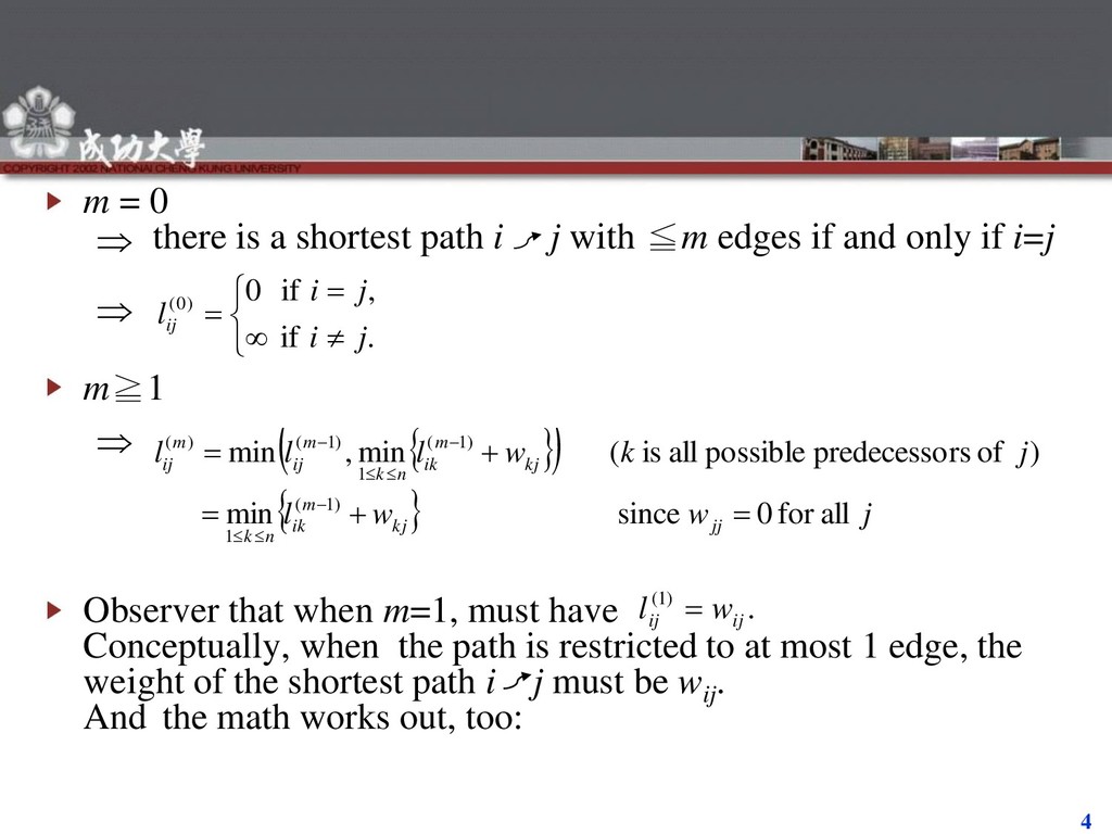
4. 4 m = 0 there is a shortest path i j with ≦m edges if and only if i=j m≧1 Observer that when m=1, must have Conceptually, when the path is restricted to at most 1 edge, the weight of the shortest path i j must be wij . And the math works out, too:          . if , if 0 ) 0 ( j i j i l ij        j w w l j k w l l l jj kj m ik n k kj m ik n k m ij m ij all for 0 since min ) of rs predecesso possible all is ( min , min ) 1 ( 1 ) 1 ( 1 ) 1 ( ) (             . ) 1 ( ij ij w l 
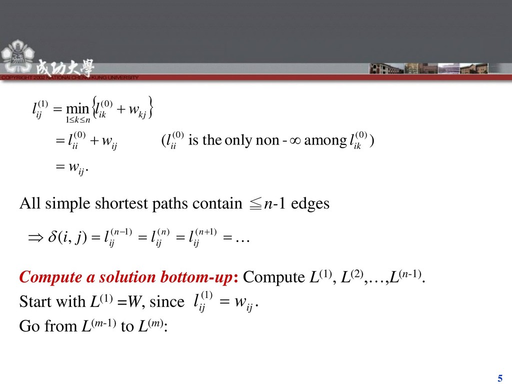
5. 5 All simple shortest paths contain ≦n-1 edges Compute a solution bottom-up: Compute L(1), L(2),…,L(n-1). Start with L(1) =W, since Go from L(m-1) to L(m):   . ) among - non only the is ( min ) 0 ( ) 0 ( ) 0 ( ) 0 ( 1 ) 1 ( ij ik ii ij ii kj ik n k ij w l l w l w l l                 ) 1 ( ) ( ) 1 ( ) , ( n ij n ij n ij l l l j i  . ) 1 ( ij ij w l 
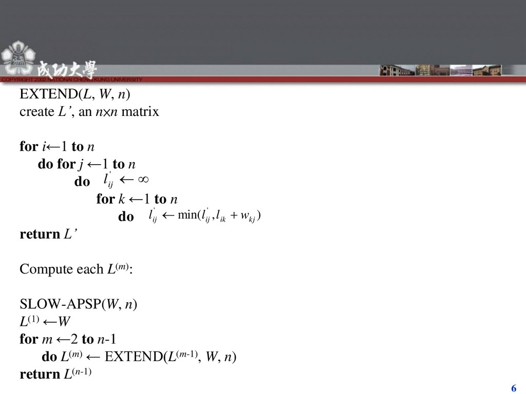
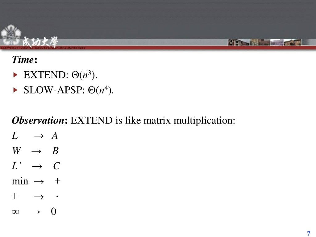
6. 6 EXTEND(L, W, n) create L’, an n×n matrix for i←1 to n do for j ←1 to n do for k ←1 to n do return L’ Compute each L(m): SLOW-APSP(W, n) L(1) ←W for m ←2 to n-1 do L(m) ← EXTEND(L(m-1), W, n) return L(n-1)   ' ij l ) , min( ' ' kj ik ij ij w l l l  
7. 7 Time: EXTEND: (n3). SLOW-APSP: (n4). Observation: EXTEND is like matrix multiplication: L → A W → B L’ → C min → + + → ． ∞ → 0
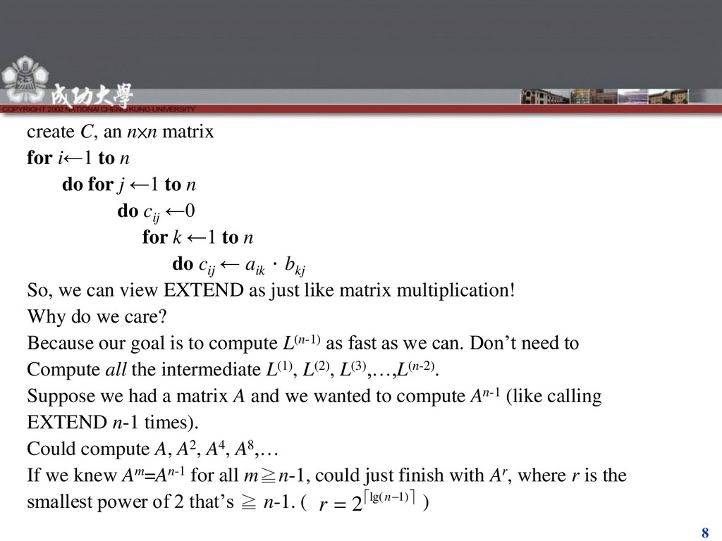
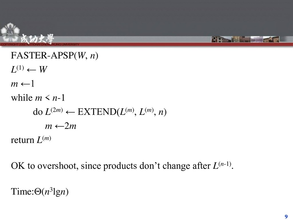
8. 8 create C, an n×n matrix for i←1 to n do for j ←1 to n do cij ←0 for k ←1 to n do cij ← aik ．bkj So, we can view EXTEND as just like matrix multiplication! Why do we care? Because our goal is to compute L(n-1) as fast as we can. Don’t need to Compute all the intermediate L(1), L(2), L(3),…,L(n-2). Suppose we had a matrix A and we wanted to compute An-1 (like calling EXTEND n-1 times). Could compute A, A2, A4, A8,… If we knew Am=An-1 for all m≧n-1, could just finish with Ar, where r is the smallest power of 2 that’s ≧ n-1. ( )   ) 1 lg( 2   n r
9. 9 FASTER-APSP(W, n) L(1) ← W m ←1 while m < n-1 do L(2m) ← EXTEND(L(m), L(m), n) m ←2m return L(m) OK to overshoot, since products don’t change after L(n-1). Time:(n3lgn)
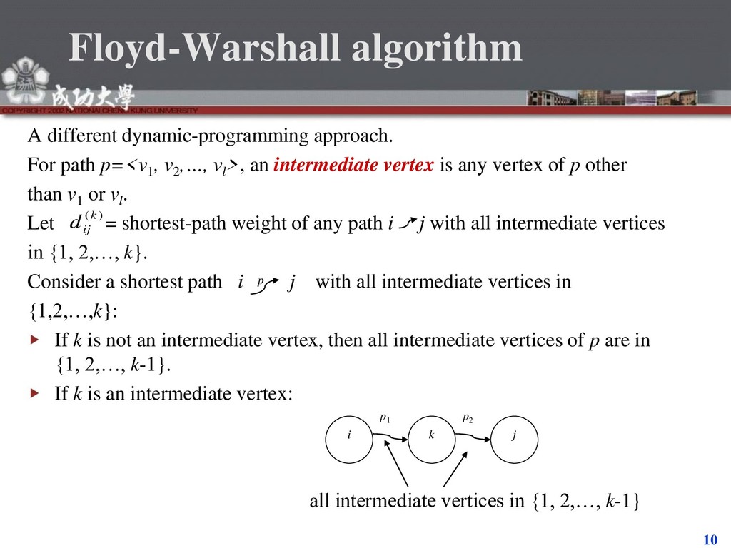
10. 10 Floyd-Warshall algorithm A different dynamic-programming approach. For path p=<v1 , v2 ,…, vl >, an intermediate vertex is any vertex of p other than v1 or vl . Let = shortest-path weight of any path i j with all intermediate vertices in {1, 2,…, k}. Consider a shortest path i j with all intermediate vertices in {1,2,…,k}: If k is not an intermediate vertex, then all intermediate vertices of p are in {1, 2,…, k-1}. If k is an intermediate vertex: ) (k ij d p i k j p1 p2 all intermediate vertices in {1, 2,…, k-1}
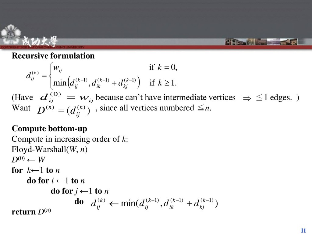
11. 11 Recursive formulation (Have because can’t have intermediate vertices ≦1 edges. ) Want , since all vertices numbered ≦n. Compute bottom-up Compute in increasing order of k: Floyd-Warshall(W, n) D(0) ← W for k←1 to n do for i ←1 to n do for j ←1 to n do return D(n)               1. if , min 0, if ) 1 ( ) 1 ( ) 1 ( ) ( k d d d k w d k kj k ik k ij ij k ij ij ij w d  ) 0 (  ) ( ) ( ) ( n ij n d D  ) , min( ) 1 ( ) 1 ( ) 1 ( ) (      k kj k ik k ij k ij d d d d
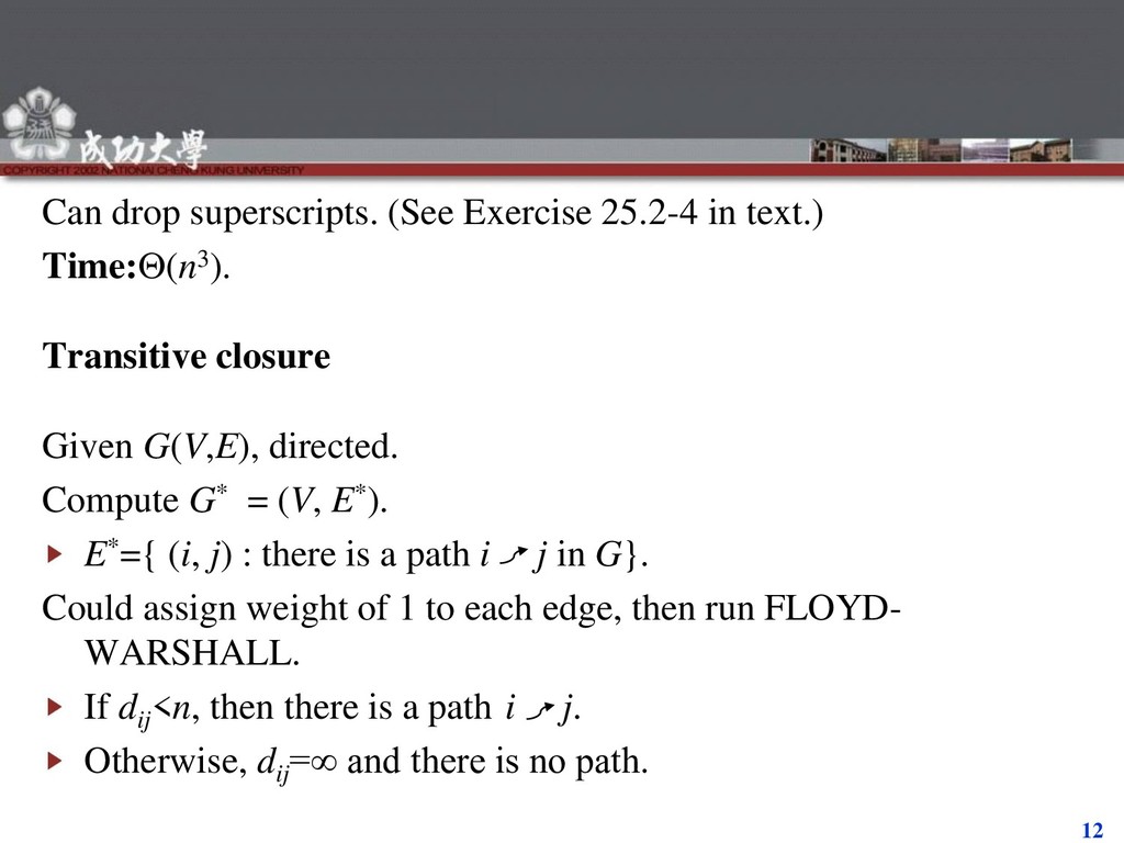
12. 12 Can drop superscripts. (See Exercise 25.2-4 in text.) Time:(n3). Transitive closure Given G(V,E), directed. Compute G* = (V, E*). E*={ (i, j) : there is a path i j in G}. Could assign weight of 1 to each edge, then run FLOYD- WARSHALL. If dij <n, then there is a path i j. Otherwise, dij =∞ and there is no path.
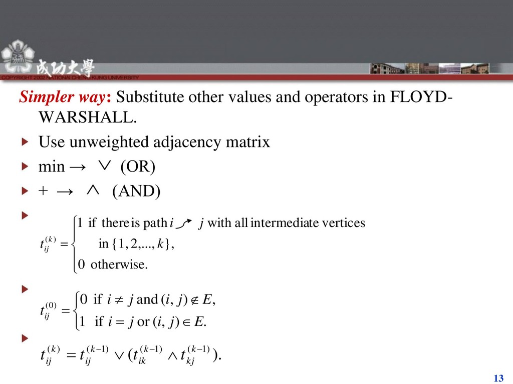
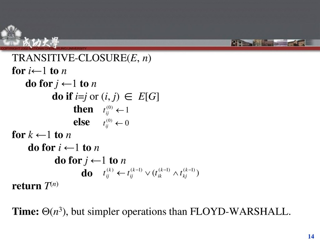
13. 13 Simpler way: Substitute other values and operators in FLOYD- WARSHALL. Use unweighted adjacency matrix min → (OR) + → (AND)       otherwise. 0 }, 2,..., {1, in vertices te intermedia all with path is there if 1 ) ( k j i t k ij         . ) , ( or if 1 , ) , ( and if 0 ) 0 ( E j i j i E j i j i t ij ). ( ) 1 ( ) 1 ( ) 1 ( ) (       k kj k ik k ij k ij t t t t  
14. 14 TRANSITIVE-CLOSURE(E, n) for i←1 to n do for j ←1 to n do if i=j or (i, j) E[G] then else for k ←1 to n do for i ←1 to n do for j ←1 to n do return T(n) Time: (n3), but simpler operations than FLOYD-WARSHALL.  1 ) 0 (  ij t 0 ) 0 (  ij t ) ( ) 1 ( ) 1 ( ) 1 ( ) (       k kj k ik k ij k ij t t t t
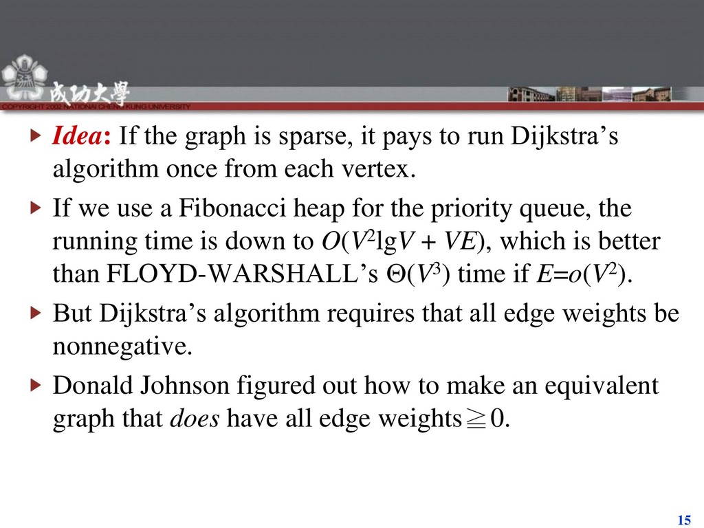
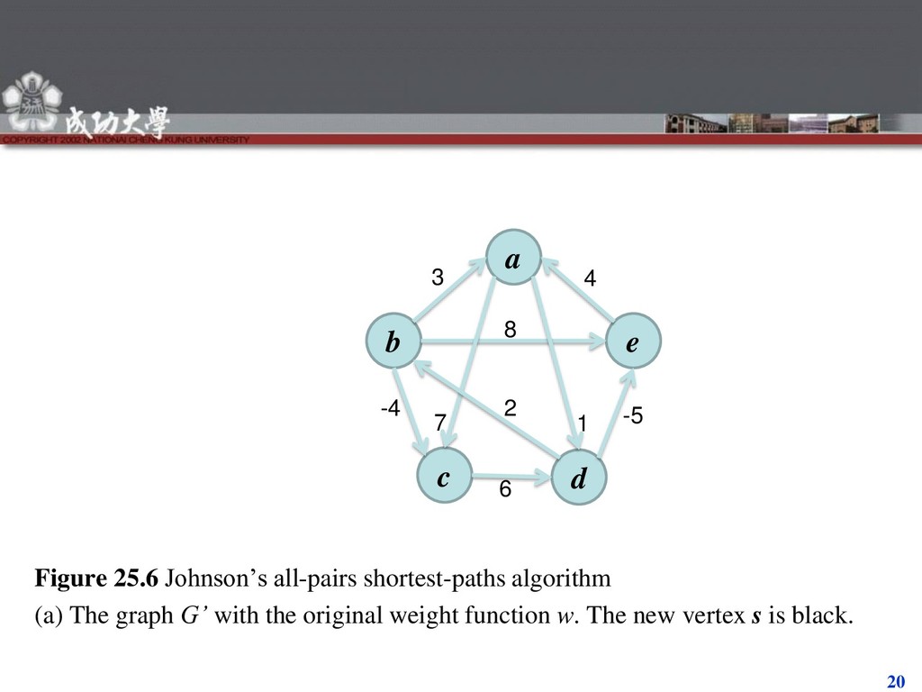
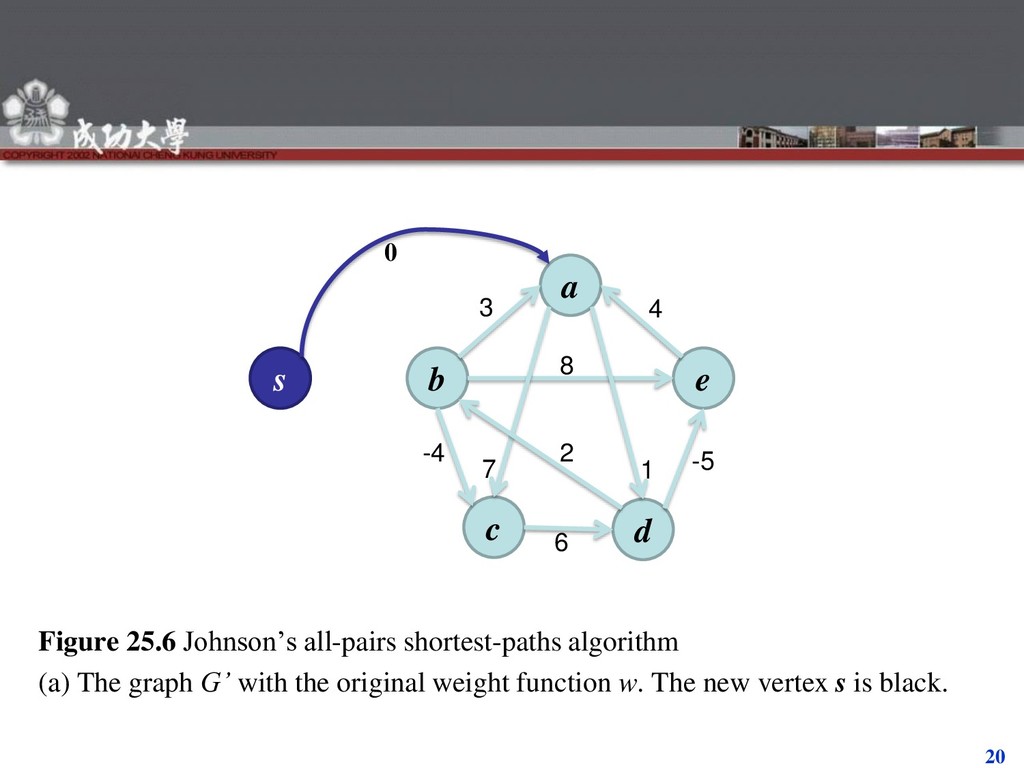
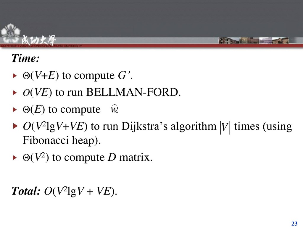
15. 15 Idea: If the graph is sparse, it pays to run Dijkstra’s algorithm once from each vertex. If we use a Fibonacci heap for the priority queue, the running time is down to O(V2lgV + VE), which is better than FLOYD-WARSHALL’s (V3) time if E=o(V2). But Dijkstra’s algorithm requires that all edge weights be nonnegative. Donald Johnson figured out how to make an equivalent graph that does have all edge weights≧0.
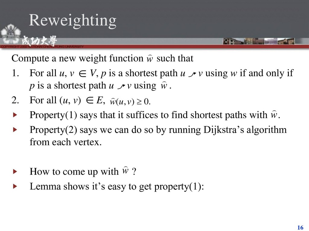
16. 16 Reweighting Compute a new weight function such that 1. For all u, v V, p is a shortest path u v using w if and only if p is a shortest path u v using . 2. For all (u, v) E, Property(1) says that it suffices to find shortest paths with . Property(2) says we can do so by running Dijkstra’s algorithm from each vertex. How to come up with ? Lemma shows it’s easy to get property(1): w   w   . 0 ) , (  v u w  w  w 
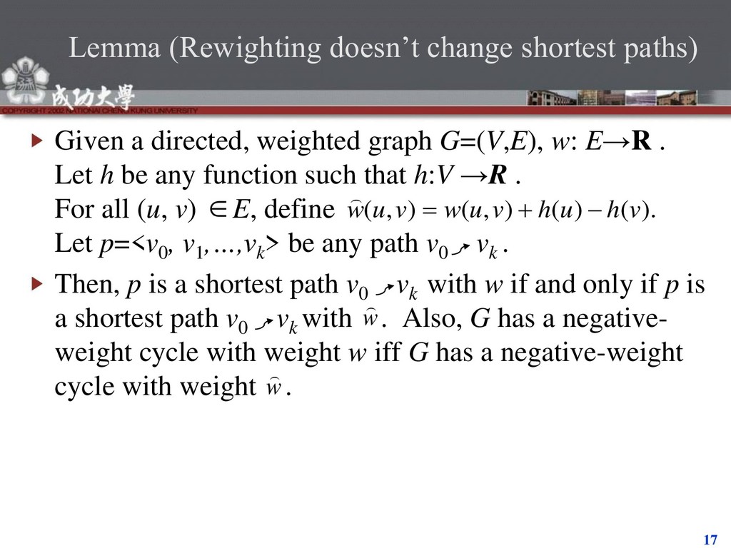
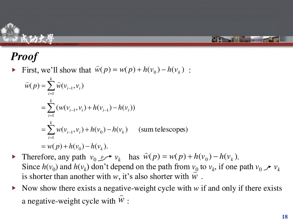
17. 17 Lemma (Rewighting doesn’t change shortest paths) Given a directed, weighted graph G=(V,E), w: E→R . Let h be any function such that h:V →R . For all (u, v) E, define Let p=<v0 , v1 ,…,vk > be any path v0 vk . Then, p is a shortest path v0 vk with w if and only if p is a shortest path v0 vk with . Also, G has a negative- weight cycle with weight w iff G has a negative-weight cycle with weight .  ). ( ) ( ) , ( ) , ( v h u h v u w v u w     w  w 
18. 18 Proof First, we’ll show that : Therefore, any path v0 vk has . Since h(v0 ) and h(vk ) don’t depend on the path from v0 to vk , if one path v0 vk is shorter than another with w, it’s also shorter with . Now show there exists a negative-weight cycle with w if and only if there exists a negative-weight cycle with : ) ( ) ( ) ( ) ( 0 k v h v h p w p w     ). ( ) ( ) ( s) telescope (sum ) ( ) ( ) , ( )) ( ) ( ) , ( ( ) , ( ) ( 0 1 0 1 1 1 1 1 1 k k i k i i k i i i i i k i i i v h v h p w v h v h v v w v h v h v v w v v w p w                       p ) ( ) ( ) ( ) ( 0 k v h v h p w p w     w  w 
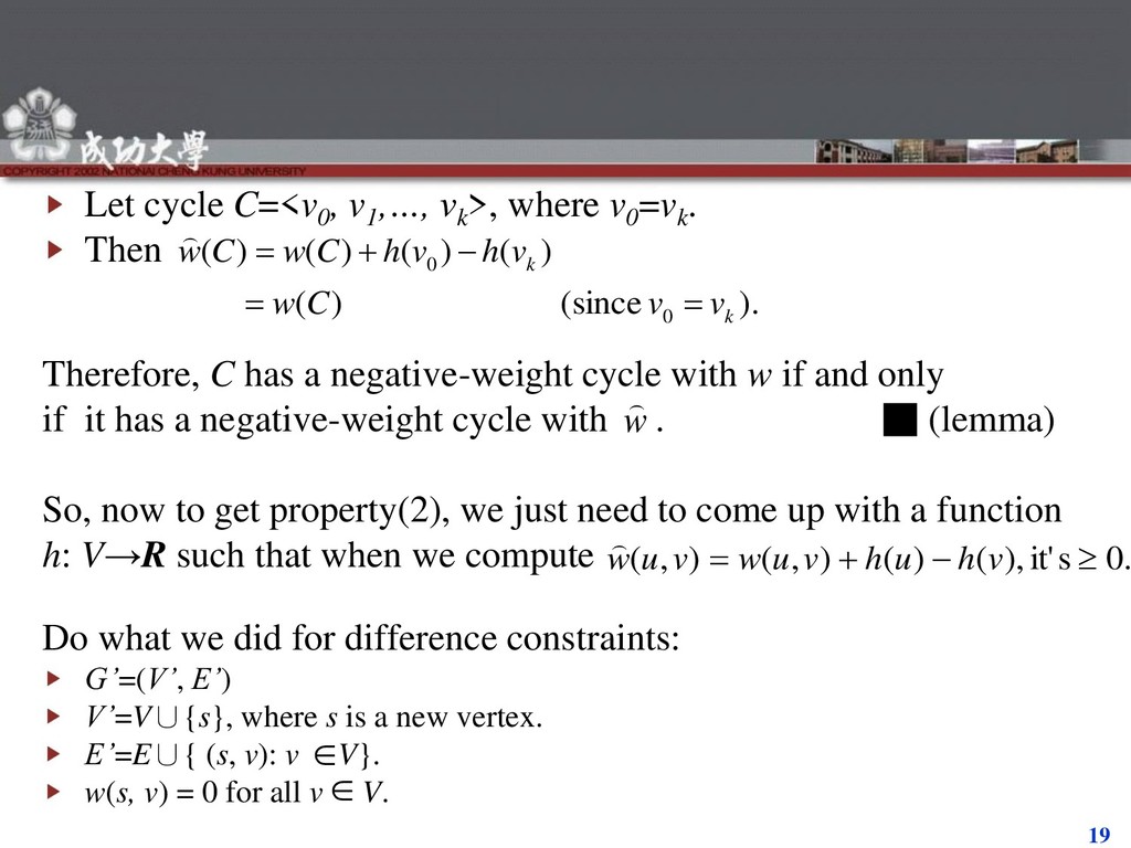
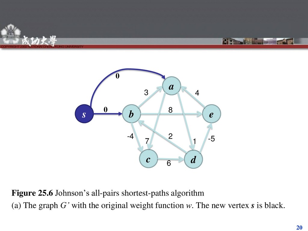
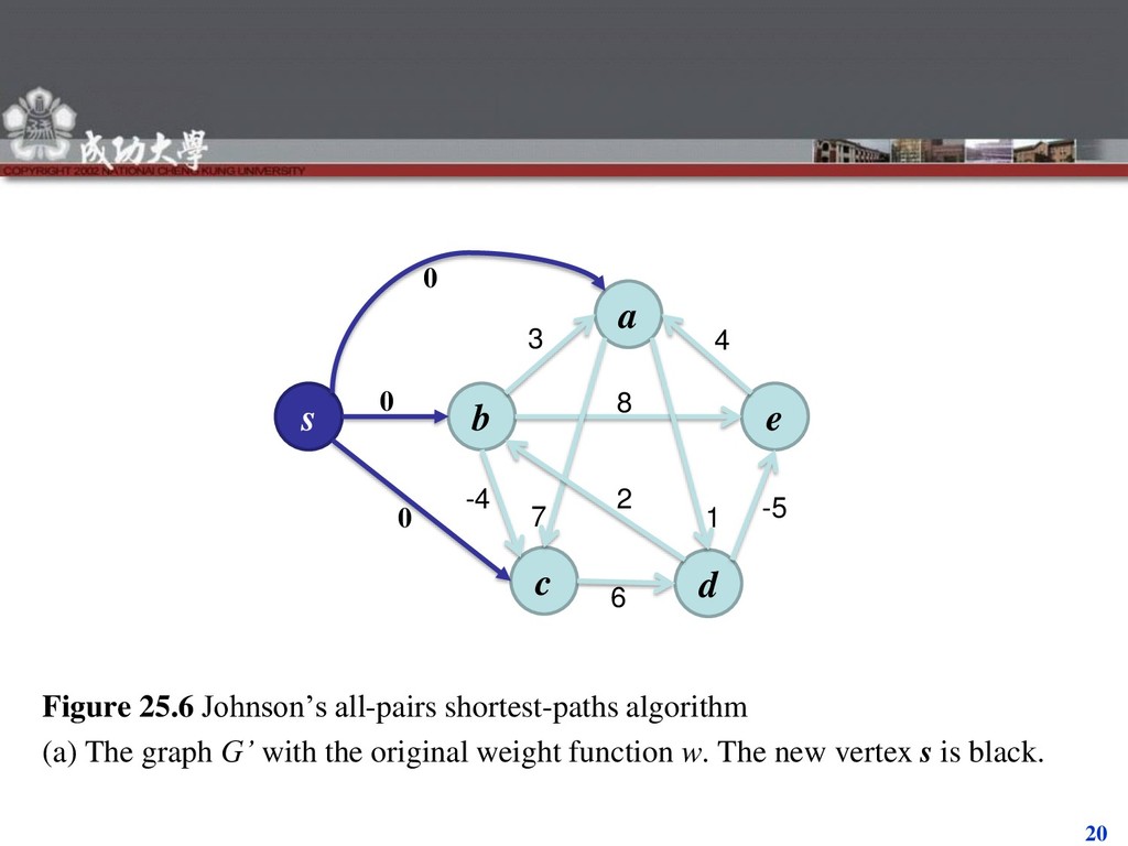
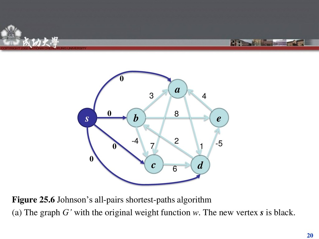
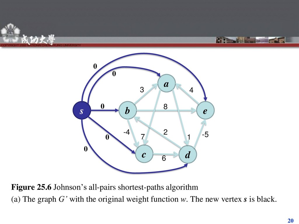
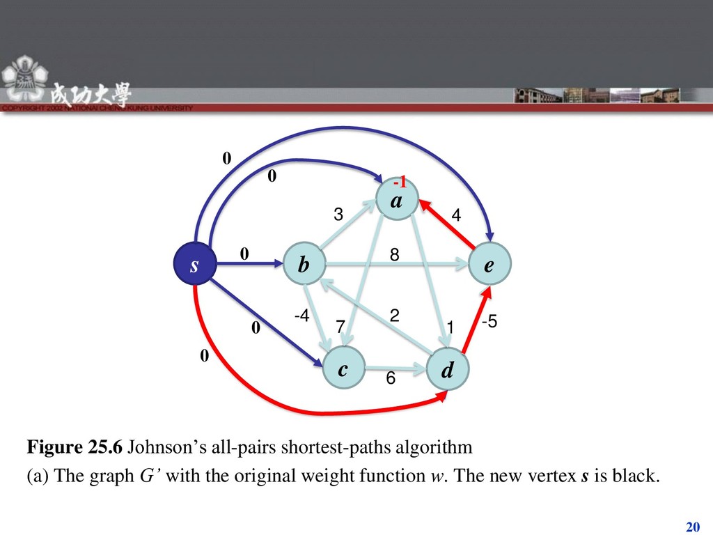
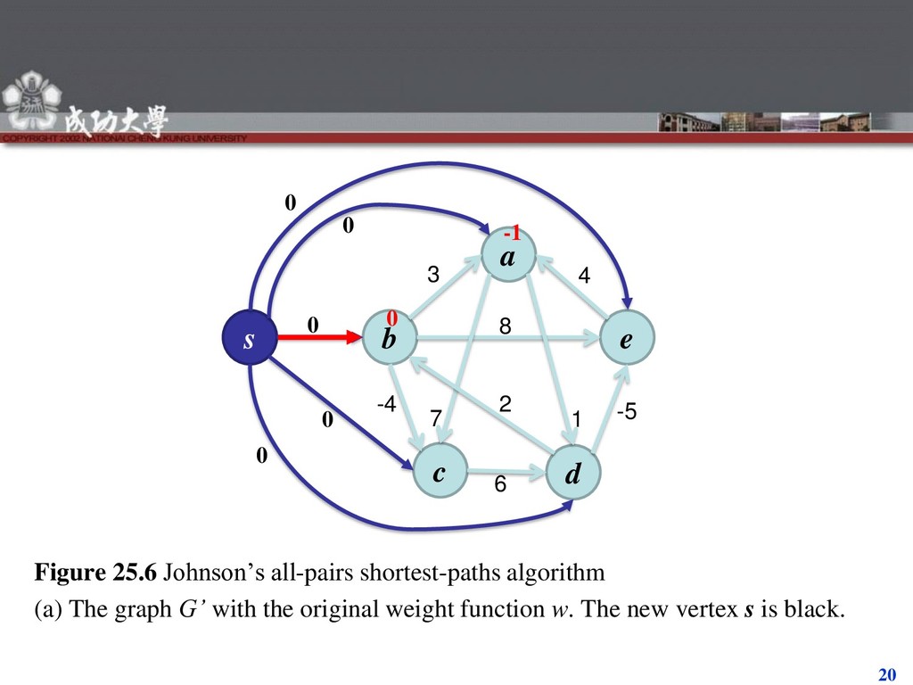
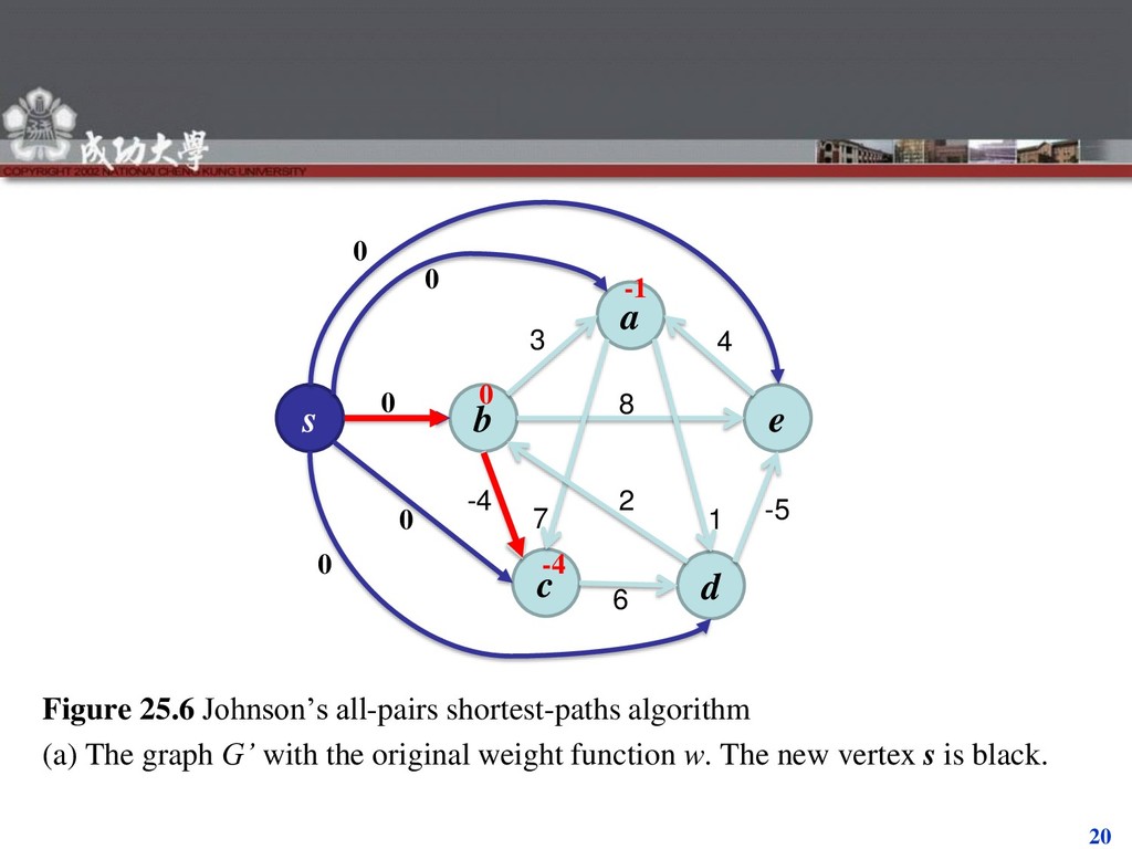
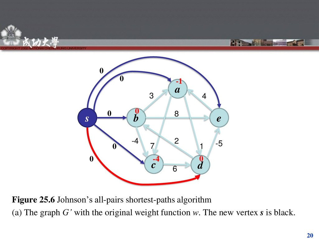
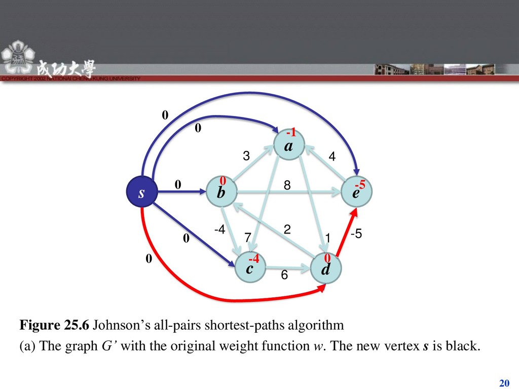
19. 19 Let cycle C=<v0 , v1 ,…, vk >, where v0 =vk . Then Therefore, C has a negative-weight cycle with w if and only if it has a negative-weight cycle with . ▪ (lemma) So, now to get property(2), we just need to come up with a function h: V→R such that when we compute Do what we did for difference constraints: G’=(V’, E’) V’=V∪{s}, where s is a new vertex. E’=E∪{ (s, v): v V}. w(s, v) = 0 for all v V. ). (since ) ( ) ( ) ( ) ( ) ( 0 0 k k v v C w v h v h C w C w       w  . 0 s it' ), ( ) ( ) , ( ) , (     v h u h v u w v u w   
20. Figure 25.6 Johnson’s all-pairs shortest-paths algorithm (a) The graph G’ with the original weight function w. The new vertex s is black. 20 a b e d c 3 -4 6 -5 4 8 2 7 1
21. Figure 25.6 Johnson’s all-pairs shortest-paths algorithm (a) The graph G’ with the original weight function w. The new vertex s is black. 20 s a b e d c 3 -4 6 -5 4 8 2 7 1
22. Figure 25.6 Johnson’s all-pairs shortest-paths algorithm (a) The graph G’ with the original weight function w. The new vertex s is black. 20 s a b e d c 3 -4 6 -5 4 8 2 7 1 0
23. Figure 25.6 Johnson’s all-pairs shortest-paths algorithm (a) The graph G’ with the original weight function w. The new vertex s is black. 20 s a b e d c 3 -4 6 -5 4 8 2 7 1 0 0
24. Figure 25.6 Johnson’s all-pairs shortest-paths algorithm (a) The graph G’ with the original weight function w. The new vertex s is black. 20 s a b e d c 3 -4 6 -5 4 8 2 7 1 0 0 0
25. Figure 25.6 Johnson’s all-pairs shortest-paths algorithm (a) The graph G’ with the original weight function w. The new vertex s is black. 20 s a b e d c 3 -4 6 -5 4 8 2 7 1 0 0 0 0
26. Figure 25.6 Johnson’s all-pairs shortest-paths algorithm (a) The graph G’ with the original weight function w. The new vertex s is black. 20 s a b e d c 3 -4 6 -5 4 8 2 7 1 0 0 0 0 0
27. Figure 25.6 Johnson’s all-pairs shortest-paths algorithm (a) The graph G’ with the original weight function w. The new vertex s is black. 20 s a b e d c 3 -4 6 -5 4 8 2 7 1 0 0 0 0 0 -1
28. Figure 25.6 Johnson’s all-pairs shortest-paths algorithm (a) The graph G’ with the original weight function w. The new vertex s is black. 20 s a b e d c 3 -4 6 -5 4 8 2 7 1 0 0 0 0 0 -1 0
29. Figure 25.6 Johnson’s all-pairs shortest-paths algorithm (a) The graph G’ with the original weight function w. The new vertex s is black. 20 s a b e d c 3 -4 6 -5 4 8 2 7 1 0 0 0 0 0 -1 -4 0
30. Figure 25.6 Johnson’s all-pairs shortest-paths algorithm (a) The graph G’ with the original weight function w. The new vertex s is black. 20 s a b e d c 3 -4 6 -5 4 8 2 7 1 0 0 0 0 0 -1 -4 0 0
31. Figure 25.6 Johnson’s all-pairs shortest-paths algorithm (a) The graph G’ with the original weight function w. The new vertex s is black. 20 s a b e d c 3 -4 6 -5 4 8 2 7 1 0 0 0 0 0 -1 -4 0 -5 0
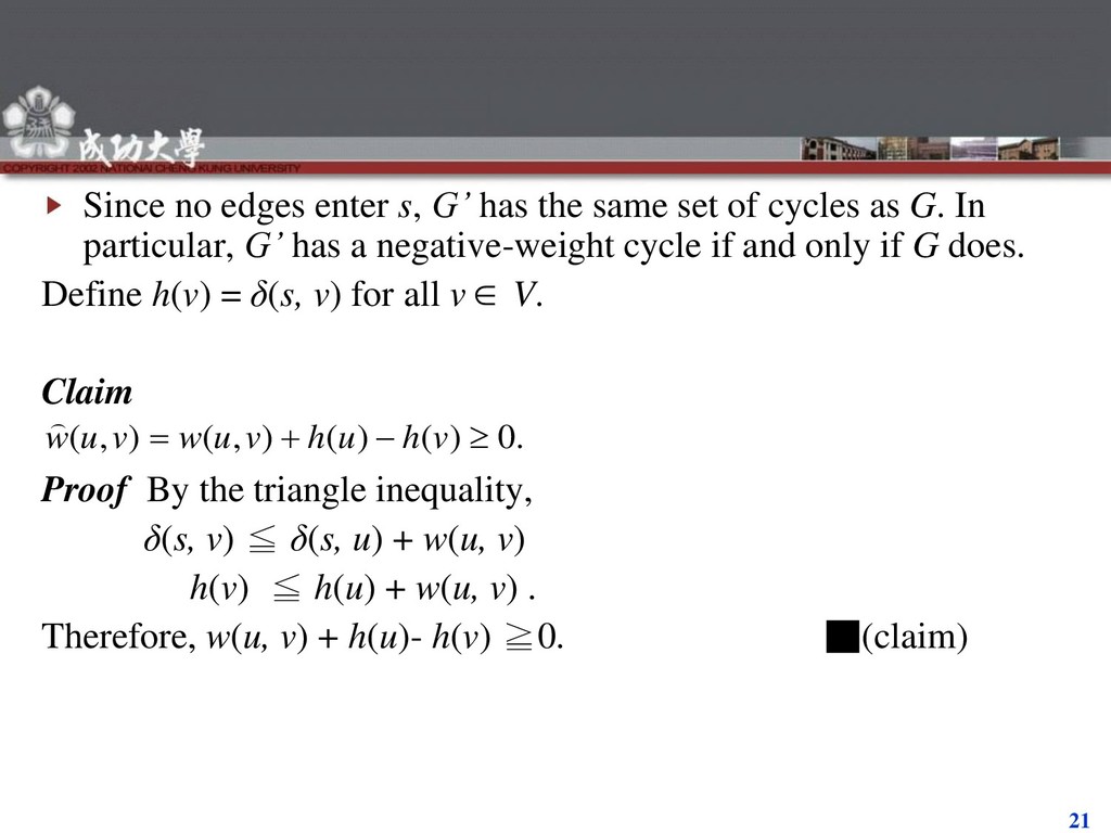
32. 21 Since no edges enter s, G’ has the same set of cycles as G. In particular, G’ has a negative-weight cycle if and only if G does. Define h(v) = δ(s, v) for all v V. Claim Proof By the triangle inequality, δ(s, v) ≦ δ(s, u) + w(u, v) h(v) ≦ h(u) + w(u, v) . Therefore, w(u, v) + h(u)- h(v) ≧0. ▪(claim)  . 0 ) ( ) ( ) , ( ) , (     v h u h v u w v u w 
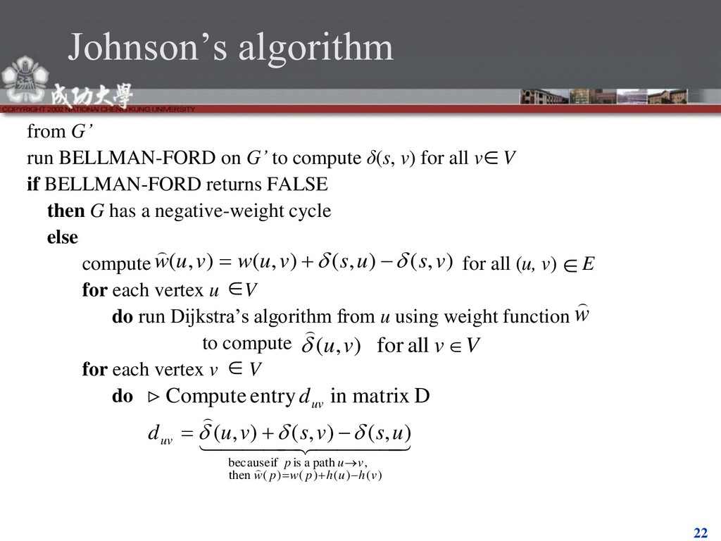
33. 22 Johnson’s algorithm from G’ run BELLMAN-FORD on G’ to compute δ(s, v) for all v V if BELLMAN-FORD returns FALSE then G has a negative-weight cycle else compute for all (u, v) E for each vertex u V do run Dijkstra’s algorithm from u using weight function to compute for each vertex v V do               ) ( ) ( ) ( ) ( then , path a is if because ) , ( ) , ( ) , ( D matrix in entry Compute v h u h p w p w v u p uv uv u s v s v u d d            ) , ( ) , ( ) , ( ) , ( v s u s v u w v u w         w  V v v u  all for ) , (   
34. 23 Time: (V+E) to compute G’. O(VE) to run BELLMAN-FORD. (E) to compute . O(V2lgV+VE) to run Dijkstra’s algorithm times (using Fibonacci heap). (V2) to compute D matrix. Total: O(V2lgV + VE). w  V