Quantum Chemical Topology: Chemistry in real space

Transcript

1. Quantum Chemical Topology: Chemistry in real space ´ Angel Mart´ ın Pend´ as angel@fluor.quimica.uniovi.es M2, Madrid 2013 c ´ Angel Mart´ ın Pend´ as, 2004-2013 (1)
2. Outline 1. Introduction. 2. QTAIM quick reference guide. 3. Electron density & Atoms in Molecules. 4. QTAIM as a theory of Atoms in Molecules. 5. Interacting Quantum Atoms (IQA) & Chemical Bonds. 6. Chemical Insights from IQA. 7. Examples. c ´ Angel Mart´ ın Pend´ as, 2004-2013 (2)
3. Introduction Introduction 1. Introduction. Quantum Chemistry is now near Dirac’s reductionist goal: • Theoretical (DFT) & Computational achievements allow us to reach chemical accuracy in everyday molecules. Problems, however, if chemical insight is regarded: 1. Wavefunction information. 2. Epistemology of emergent phenomena. Chemistry has a language defined before Quantum Mechanics. • Chemists envision entities in interaction • These entities live in 3D space, and are embodied with properties: bonds, transferability, characteristic energies and reactivities... We need interpretations!. How do we extract chemically meaningful information from ? ↵ Chemistry c ´ Angel Mart´ ın Pend´ as, 2004-2013 (3)
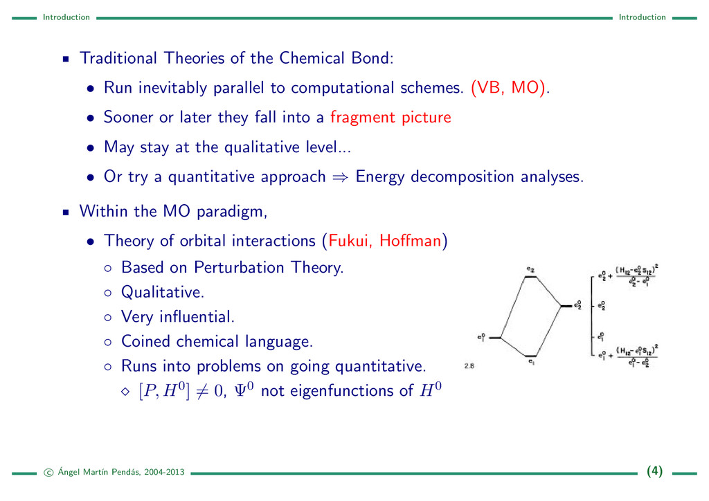
4. Introduction Introduction Traditional Theories of the Chemical Bond: • Run inevitably parallel to computational schemes. (VB, MO). • Sooner or later they fall into a fragment picture • May stay at the qualitative level... • Or try a quantitative approach ) Energy decomposition analyses. Within the MO paradigm, • Theory of orbital interactions (Fukui, Ho↵man) Based on Perturbation Theory. Qualitative. Very influential. Coined chemical language. Runs into problems on going quantitative. ⇧ [P, H0] 6= 0, 0 not eigenfunctions of H0 c ´ Angel Mart´ ın Pend´ as, 2004-2013 (4)
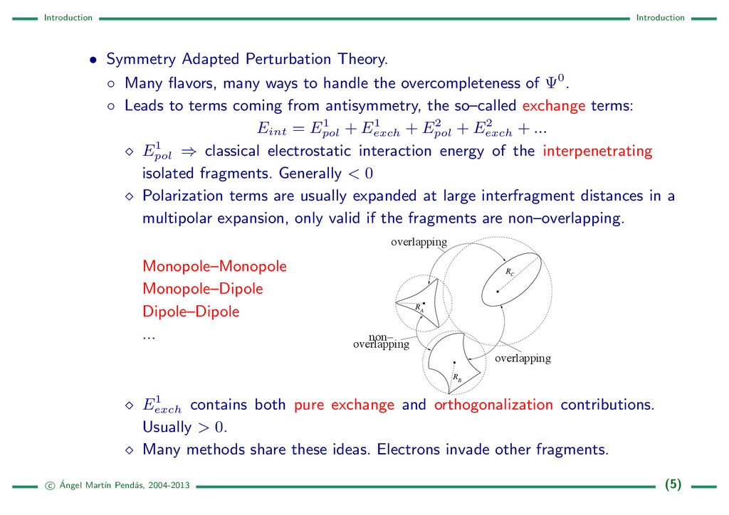
5. Introduction Introduction • Symmetry Adapted Perturbation Theory. Many flavors, many ways to handle the overcompleteness of 0. Leads to terms coming from antisymmetry, the so–called exchange terms: Eint = E1 pol + E1 exch + E2 pol + E2 exch + ... ⇧ E1 pol ) classical electrostatic interaction energy of the interpenetrating isolated fragments. Generally < 0 ⇧ Polarization terms are usually expanded at large interfragment distances in a multipolar expansion, only valid if the fragments are non–overlapping. Monopole–Monopole Monopole–Dipole Dipole–Dipole ... A R B R C non− overlapping overlapping R overlapping ⇧ E1 exch contains both pure exchange and orthogonalization contributions. Usually > 0 . ⇧ Many methods share these ideas. Electrons invade other fragments. c ´ Angel Mart´ ın Pend´ as, 2004-2013 (5)
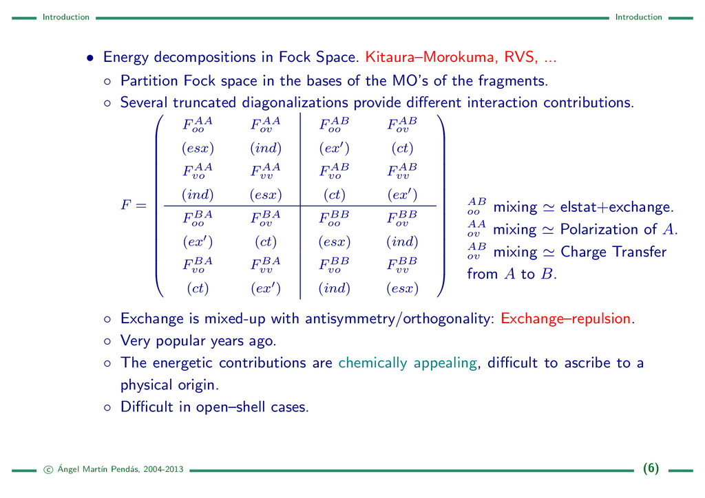
6. Introduction Introduction • Energy decompositions in Fock Space. Kitaura–Morokuma, RVS, ... Partition Fock space in the bases of the MO’s of the fragments. Several truncated diagonalizations provide di↵erent interaction contributions. F = 0 B B B B B B B B B B B B B B B B @ FAA oo (esx) FAA ov (ind) FAB oo (ex0) FAB ov (ct) FAA vo (ind) FAA vv (esx) FAB vo (ct) FAB vv (ex0) FBA oo (ex0) FBA ov (ct) FBB oo (esx) FBB ov (ind) FBA vo (ct) FBA vv (ex0) FBB vo (ind) FBB vv (esx) 1 C C C C C C C C C C C C C C C C A Exchange is mixed-up with antisymmetry/orthogonality: Exchange–repulsion. Very popular years ago. The energetic contributions are chemically appealing, di cult to ascribe to a physical origin. Di cult in open–shell cases. AB oo mixing ' elstat+exchange. AA ov mixing ' Polarization of A. AB ov mixing ' Charge Transfer from A to B. c ´ Angel Mart´ ın Pend´ as, 2004-2013 (6)
7. Introduction Introduction • Ziegler–Rauk like Energy Decompositions. Mixed scheme based on physical & chemical ideas. Molecule Formation ' Preparation + electrostatics + antisymmetrization + orbital interaction. 0 A 0 B ! 0⇤ A 0⇤ B ! A 0⇤ A 0⇤ B = 0⇤ AB ! AB E int = E prep + E elstat + E P auli rep + E orb int Antisymmetrization/Orthogonalization of the fragments ) Kinetic energy. Particular orbital contributions may be isolated. May be applied to general open–shell cases. Similar situation in the VB paradigm. Criticism: • Generality, linkage to calculational procedure. • Dependence on the reference. • Use of fictitious intermediate states. • Exchange included in/mixed-up with orthogonality. c ´ Angel Mart´ ın Pend´ as, 2004-2013 (7)
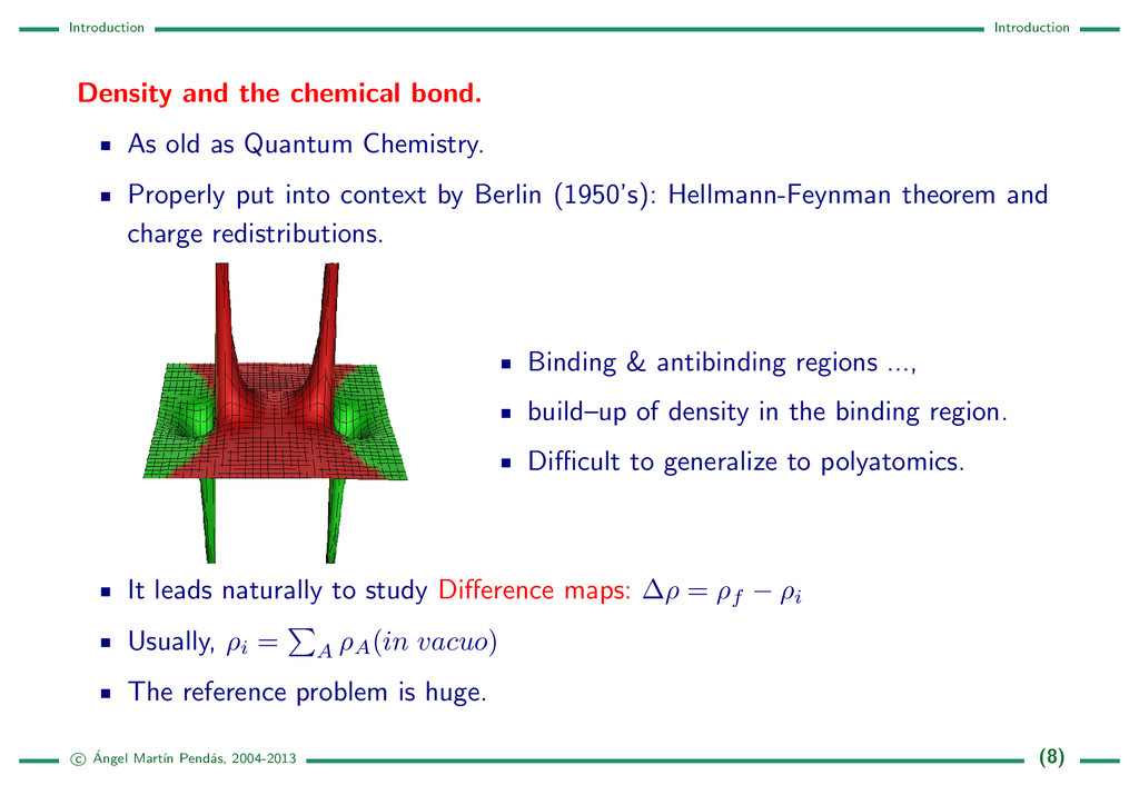
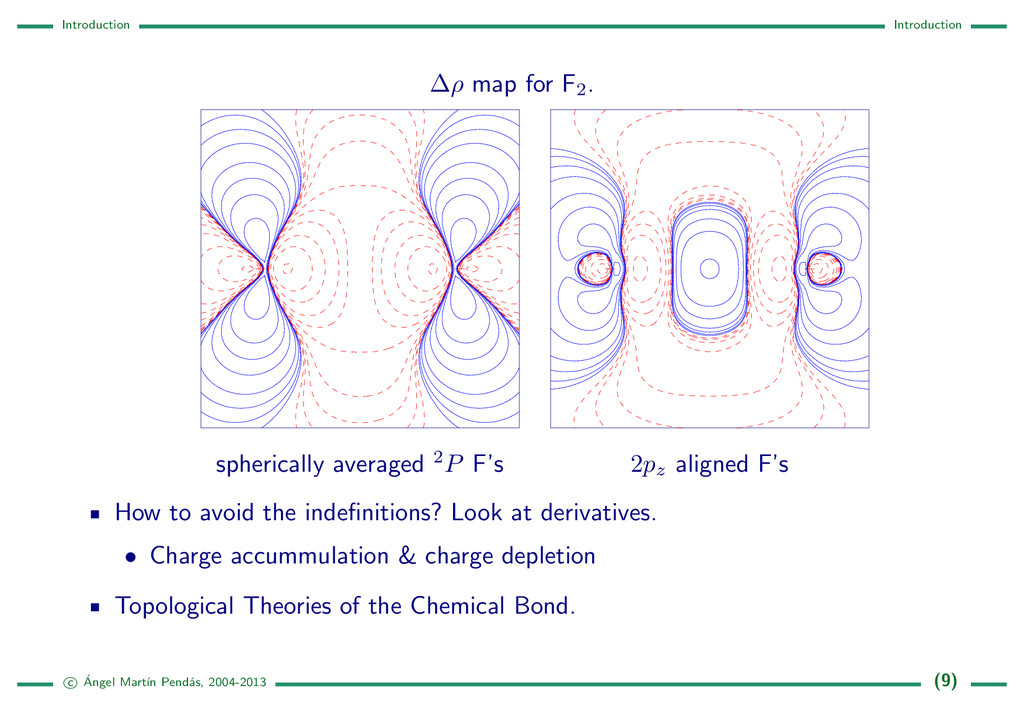
8. Introduction Introduction Density and the chemical bond. As old as Quantum Chemistry. Properly put into context by Berlin (1950’s): Hellmann-Feynman theorem and charge redistributions. Binding & antibinding regions ..., build–up of density in the binding region. Di cult to generalize to polyatomics. It leads naturally to study Di↵erence maps: ⇢ = ⇢ f ⇢ i Usually, ⇢ i = P A ⇢ A (in vacuo) The reference problem is huge. c ´ Angel Mart´ ın Pend´ as, 2004-2013 (8)
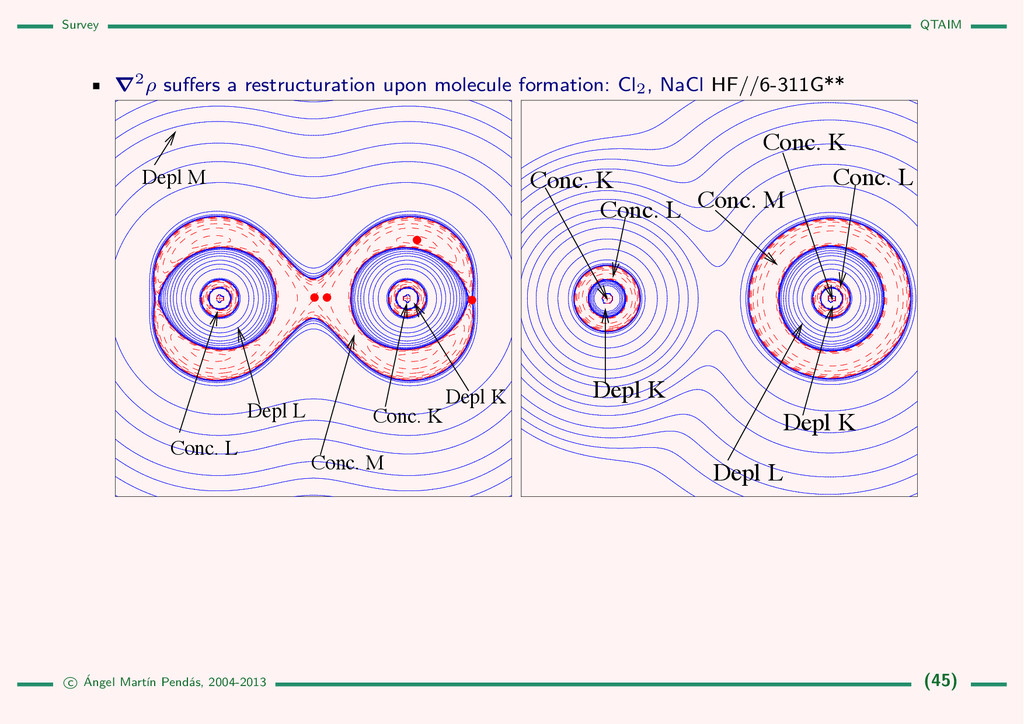
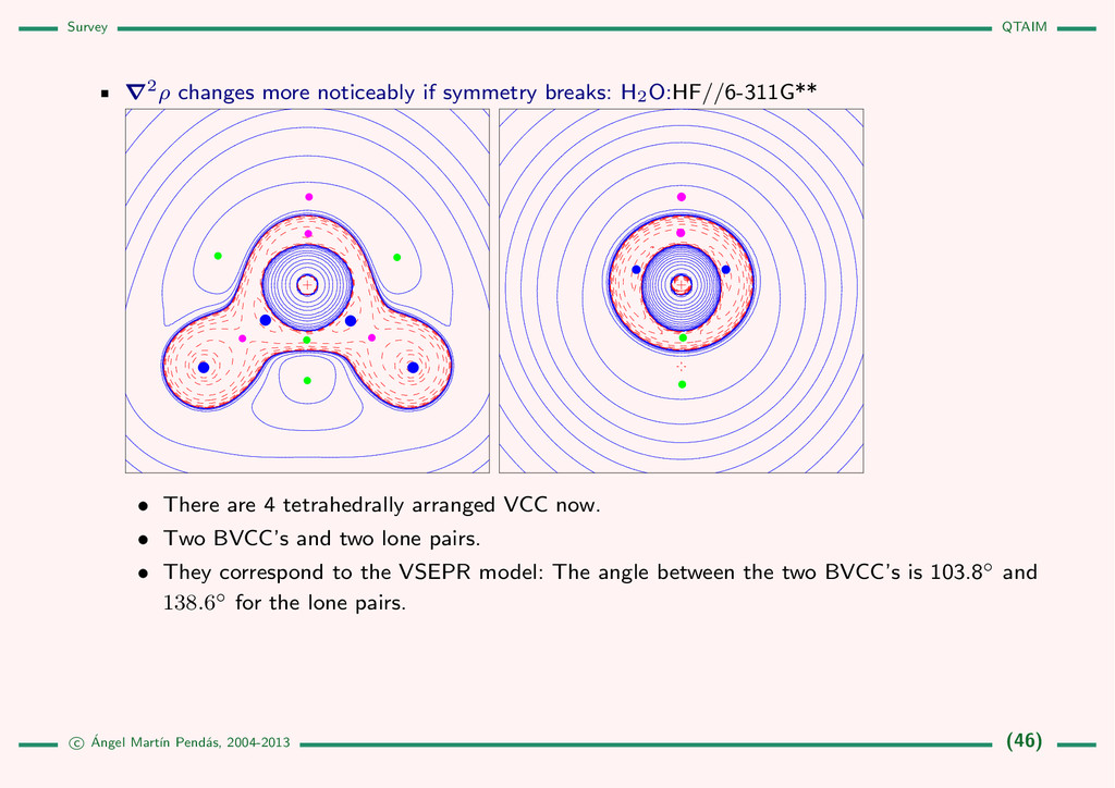
9. Introduction Introduction ⇢ map for F2. spherically averaged 2P F’s 2p z aligned F’s How to avoid the indefinitions? Look at derivatives. • Charge accummulation & charge depletion Topological Theories of the Chemical Bond. c ´ Angel Mart´ ın Pend´ as, 2004-2013 (9)
10. Introduction Introduction The topology induced by many scalar fields constructed from reduced density matrices carry chemical information 1. Take a scalar field f : D ! R 2. Construct its gradient field: rf 3. Obtain its CPs, isolate local maxima (M) or minima (m). 4. Build their attraction or repulsion basins: D = S M ( m ) D M ( m ) A number of them, according to the scalar studied: (⇢, ELF, ...) QTAIM is based on the attraction basins of ⇢. • Part of many standard chemistry curricula. Many advocates and detractors. • The topological method integrates: A theory without external references. An exhaustive partition of the 3D space. A method to obtain binary relations between chemical objects. c ´ Angel Mart´ ın Pend´ as, 2004-2013 (10)
11. Introduction Introduction • The topological method achieves: A theory of bonding: The CP’s carry chemical information A theory of atoms in molecules, and groups of atoms or functional groups. An additive partition of observables into basin contributions: h ˆ O⌦ i = R ⌦ ˆ o(r)dr • Problems with a theory of binding. Objective: a quantitative theory of binding based on the density. • Living in the 3D space. • Free of references. • Providing an exact partition of the density. • Providing an exact partition of the energy. • Consistent with conventional wisdom. • Whose terms display a clear physical interpretation. c ´ Angel Mart´ ın Pend´ as, 2004-2013 (11)
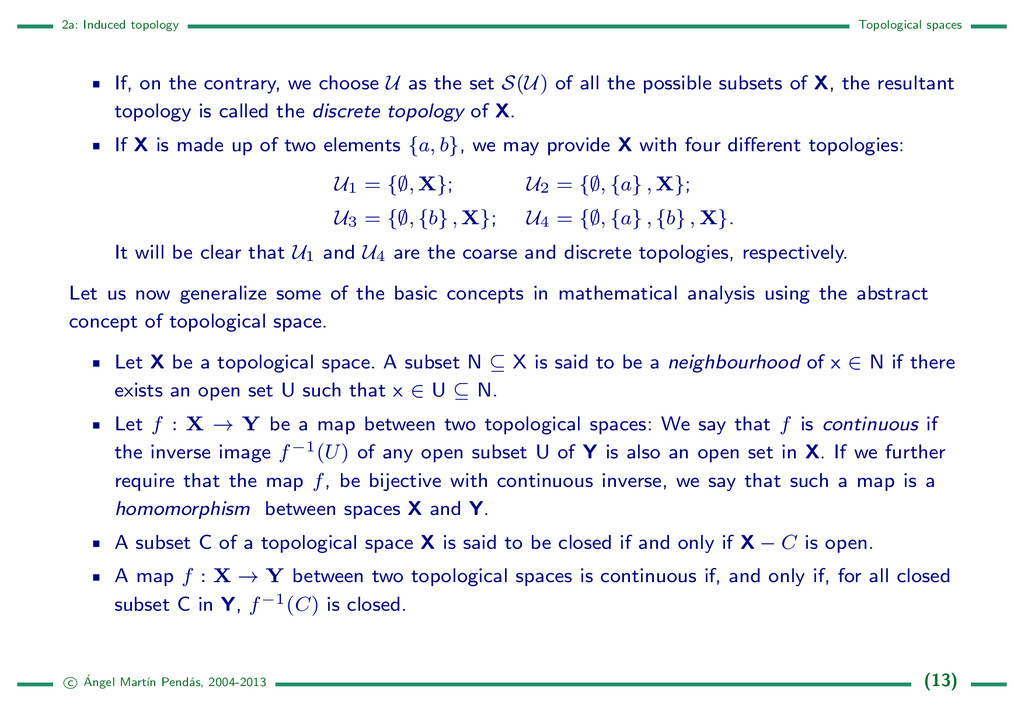
12. 2a: Induced topology Topological spaces Topological Spaces The concept of topological space is introduced so that the notion of continuity is extended to more general sets of objects. A Topology associated to a set of objects X, is a collection U of subsets of X that satisfy the following conditions: ; 2 U, X 2 U, The intersection of any two members of U is also in U, The union of any number of members of U belongs to U. -The set X , together with the collection of subsets U, define a topological space denoted as (X, U). -The members U 2 U are called open sets of the topological space X. -Every topology over a set carries an associated partition into subsets. A topology defined on the physical space provides a partition of R3. Examples: If we take as U = {;, X}, that is, the empty and the full sets, then, obviously, these comply with the axioms that define a topological space. This topology, that may be defined in any space X is called the coarse or indiscrete topology of X. c ´ Angel Mart´ ın Pend´ as, 2004-2013 (12)
13. 2a: Induced topology Topological spaces If, on the contrary, we choose U as the set S(U) of all the possible subsets of X, the resultant topology is called the discrete topology of X. If X is made up of two elements {a, b}, we may provide X with four di↵erent topologies: U1 = {;, X }; U2 = {;, {a} , X }; U3 = {;, {b} , X }; U4 = {;, {a} , {b} , X }. It will be clear that U1 and U4 are the coarse and discrete topologies, respectively. Let us now generalize some of the basic concepts in mathematical analysis using the abstract concept of topological space. Let X be a topological space. A subset N ✓ X is said to be a neighbourhood of x 2 N if there exists an open set U such that x 2 U ✓ N. Let f : X ! Y be a map between two topological spaces: We say that f is continuous if the inverse image f 1(U) of any open subset U of Y is also an open set in X. If we further require that the map f, be bijective with continuous inverse, we say that such a map is a homomorphism between spaces X and Y. A subset C of a topological space X is said to be closed if and only if X C is open. A map f : X ! Y between two topological spaces is continuous if, and only if, for all closed subset C in Y, f 1(C) is closed. c ´ Angel Mart´ ın Pend´ as, 2004-2013 (13)
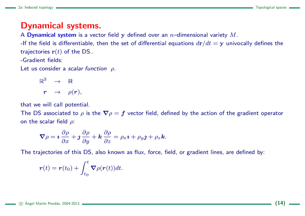
14. 2a: Induced topology Topological spaces Dynamical systems. A Dynamical system is a vector field y defined over an n–dimensional variety M. -If the field is di↵erentiable, then the set of di↵erential equations d r /dt = y univocally defines the trajectories r (t) of the DS.. -Gradient fields: Let us consider a scalar function ⇢. 3 ! r ! ⇢( r ), that we will call potential. The DS associated to ⇢ is the r⇢ = f vector field, defined by the action of the gradient operator on the scalar field ⇢: r⇢ = ı @⇢ @x + | @⇢ @y + k @⇢ @z = ⇢x ı + ⇢y | + ⇢z k . The trajectories of this DS, also known as flux, force, field, or gradient lines, are defined by: r (t) = r (t0) + Z t t 0 r⇢( r (t))dt. c ´ Angel Mart´ ın Pend´ as, 2004-2013 (14)
15. 2a: Induced topology Topological spaces Some of their properties are: 1. One and only one trajectory of r⇢ passes through any point r of the domain space. This is equivalent to saying that field trajectories of r⇢ do never cross each other. The only exception to this rule is found at the so-called critical points of the field. 2. At each point r , the vector r⇢( r ) is tangent to the field line passing through that point. 3. Given that the gradient field always points along the steepest ascent direction of ⇢, the trajectories of r⇢ are orthogonal to the isoscalar lines . 4. Each trajectory must originate or end up either at a point where r⇢( r ) = 0 , or at infinity. c ´ Angel Mart´ ın Pend´ as, 2004-2013 (15)
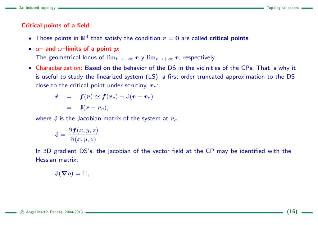
16. 2a: Induced topology Topological spaces Critical points of a field: Those points in 3 that satisfy the condition ˙ r = 0 are called critical points. ↵– and !–limits of a point p : The geometrical locus of l´ ımt! 1 r y l´ ımt!+1 r , respectively. Characterization: Based on the behavior of the DS in the vicinities of the CPs. That is why it is useful to study the linearized system (LS), a first order truncated approximation to the DS close to the critical point under scrutiny, rc: ˙ r = f ( r ) ' f ( rc) + ( r rc) = ( r rc), where is the Jacobian matrix of the system at rc, = @ f (x, y, z) @(x, y, z) . In 3D gradient DS’s, the jacobian of the vector field at the CP may be identified with the Hessian matrix: (r⇢) = , c ´ Angel Mart´ ın Pend´ as, 2004-2013 (16)
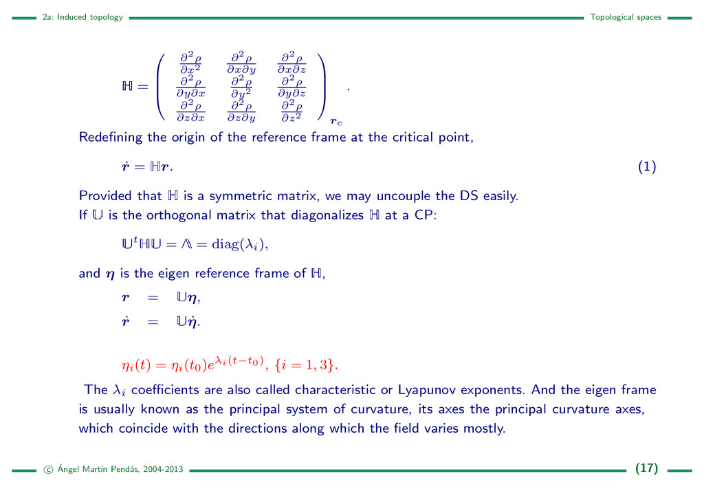
17. 2a: Induced topology Topological spaces = 0 B B @ @2⇢ @x2 @2⇢ @x@y @2⇢ @x@z @2⇢ @y@x @2⇢ @y2 @2⇢ @y@z @2⇢ @z@x @2⇢ @z@y @2⇢ @z2 1 C C A rc . Redefining the origin of the reference frame at the critical point, ˙ r = r . (1) Provided that is a symmetric matrix, we may uncouple the DS easily. If is the orthogonal matrix that diagonalizes at a CP: t = = diag( i), and ⌘ is the eigen reference frame of , r = ⌘ , ˙ r = ˙ ⌘ . ⌘i(t) = ⌘i(t0)e i(t t 0 ), {i = 1, 3}. The i coe cients are also called characteristic or Lyapunov exponents. And the eigen frame is usually known as the principal system of curvature, its axes the principal curvature axes, which coincide with the directions along which the field varies mostly. c ´ Angel Mart´ ın Pend´ as, 2004-2013 (17)
18. 2a: Induced topology Topological spaces There exist 4 di↵erent types of non-degenerate CPs in 3. In this field it is customary to classify them according to a terminology with two integer indices (r, s). The rank , r, is defined as the number of non vanishing curvatures at the CP, and the signature , s, as the di↵erence between the number of positive and negative curvatures. The set of points with field lines ending at a given CP is known as the basin of attraction of the CP. Al conjunto de puntos cuyas l´ ıneas de campo nacen en un determinado The set of points with field lines starting at a given CP is known as the basin of repulsion of the CP. c ´ Angel Mart´ ın Pend´ as, 2004-2013 (18)
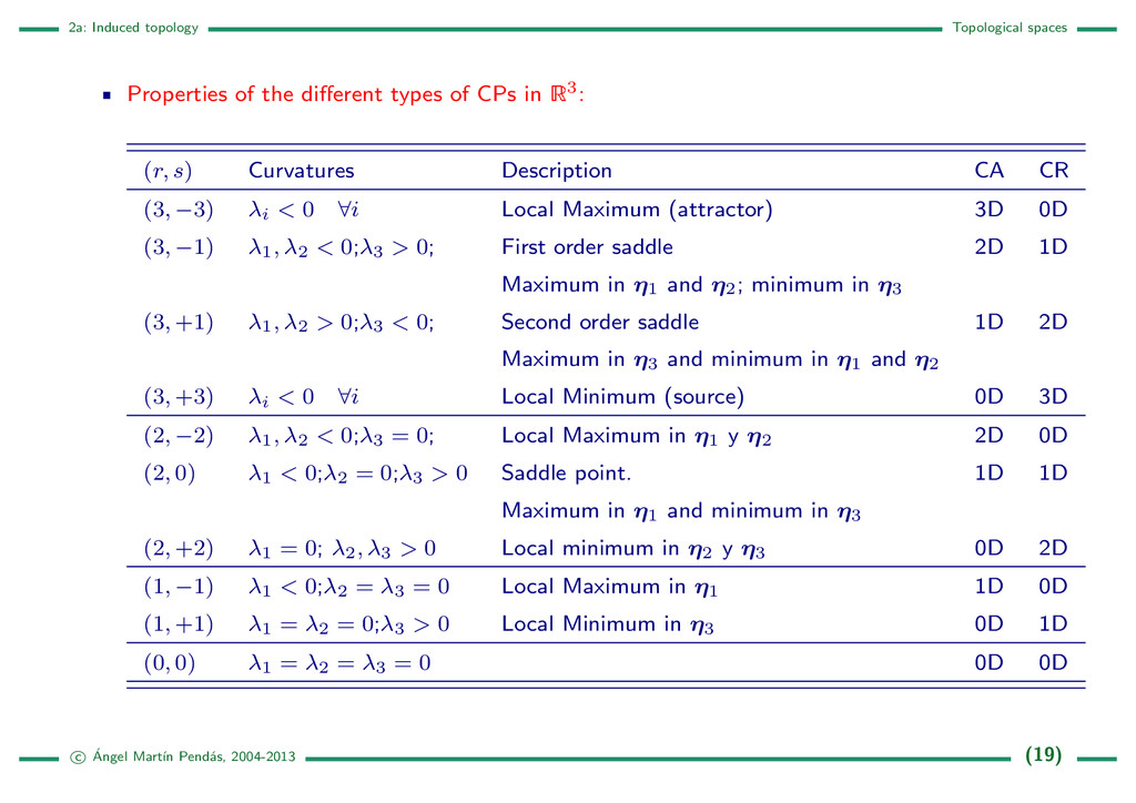
19. 2a: Induced topology Topological spaces Properties of the di↵erent types of CPs in 3: (r, s) Curvatures Description CA CR (3, 3) i < 0 8i Local Maximum (attractor) 3D 0D (3, 1) 1, 2 < 0; 3 > 0; First order saddle 2D 1D Maximum in ⌘1 and ⌘2; minimum in ⌘3 (3, +1) 1, 2 > 0; 3 < 0; Second order saddle 1D 2D Maximum in ⌘3 and minimum in ⌘1 and ⌘2 (3, +3) i < 0 8i Local Minimum (source) 0D 3D (2, 2) 1, 2 < 0; 3 = 0; Local Maximum in ⌘1 y ⌘2 2D 0D (2, 0) 1 < 0; 2 = 0; 3 > 0 Saddle point. 1D 1D Maximum in ⌘1 and minimum in ⌘3 (2, +2) 1 = 0; 2, 3 > 0 Local minimum in ⌘2 y ⌘3 0D 2D (1, 1) 1 < 0; 2 = 3 = 0 Local Maximum in ⌘1 1D 0D (1, +1) 1 = 2 = 0; 3 > 0 Local Minimum in ⌘3 0D 1D (0, 0) 1 = 2 = 3 = 0 0D 0D c ´ Angel Mart´ ın Pend´ as, 2004-2013 (19)
20. 2a: Induced topology Topological spaces Image: c ´ Angel Mart´ ın Pend´ as, 2004-2013 (20)
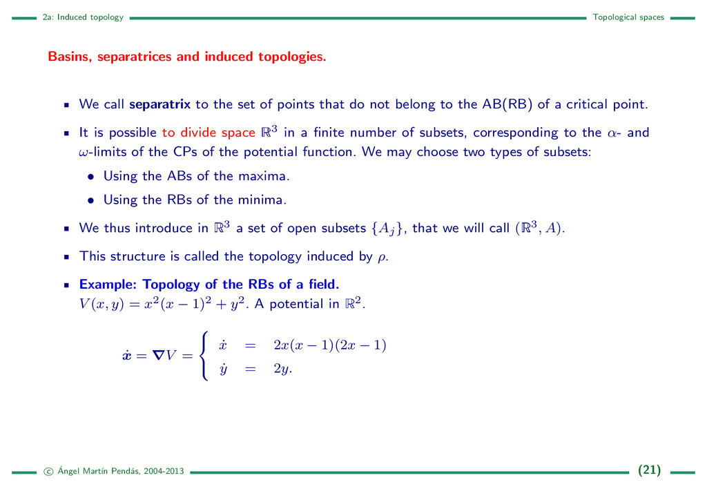
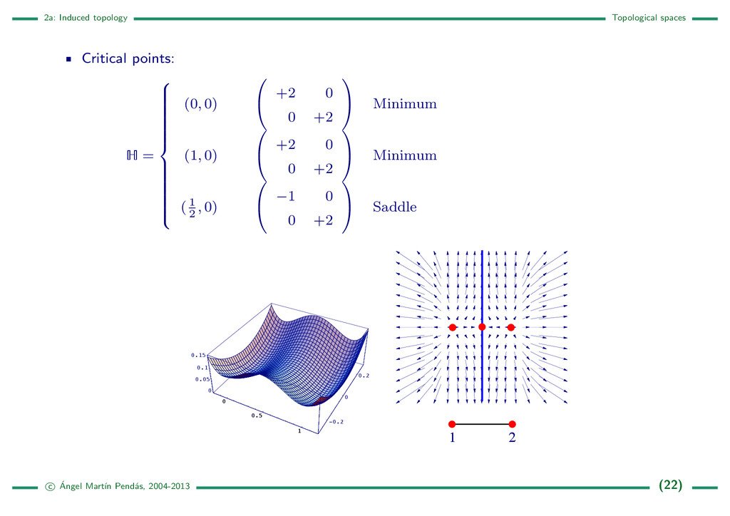
21. 2a: Induced topology Topological spaces Basins, separatrices and induced topologies. We call separatrix to the set of points that do not belong to the AB(RB) of a critical point. It is possible to divide space 3 in a finite number of subsets, corresponding to the ↵- and !-limits of the CPs of the potential function. We may choose two types of subsets: • Using the ABs of the maxima. • Using the RBs of the minima. We thus introduce in 3 a set of open subsets {Aj}, that we will call ( 3, A). This structure is called the topology induced by ⇢. Example: Topology of the RBs of a field. V (x, y) = x2(x 1)2 + y2. A potential in 2. ˙ x = rV = 8 < : ˙ x = 2x(x 1)(2x 1) ˙ y = 2y. c ´ Angel Mart´ ın Pend´ as, 2004-2013 (21)
22. 2a: Induced topology Topological spaces Critical points: = 8 > > > > > > > > > > > < > > > > > > > > > > > : (0, 0) 0 @ +2 0 0 +2 1 A Minimum (1, 0) 0 @ +2 0 0 +2 1 A Minimum ( 1 2 , 0) 0 @ 1 0 0 +2 1 A Saddle 0 0.5 1 -0.2 0 0.2 0 0.05 0.1 0.15 0 0.5 1 1 2 c ´ Angel Mart´ ın Pend´ as, 2004-2013 (22)
23. 2a: Induced topology Topological spaces The Separatrix is a local zero flux surface: Z S rV ( r ) · n ( r )ds = 0. The gradient field has generated a partition of the 2D space in three regions. A binary relationship between the two basins appears. Basin 1 is related to basin 2, since a saddle exists which AB connects both repulsors. Topological invariants. The number and type of non-degenerate critical points of a field depends on the structure of the supporting variety. For instance, in a ring, S1, the number of maxima must be equal to the number of minima. These relationships may be generalized using concepts from topology. The Betti number, Rn, of a veriety D is the number of n–dimensional topologically di↵erent regions that have no boundaries and are not boundaries of (n + 1)–dimensional regions of D. • in S1: R0 = 1, R1 = 1. • in S2: R0 = 1, R1 = 0, R2 = 1. • in T2: R0 = 1, R1 = 2, R2 = 1. • in T3: R0 = 1, R1 = 3, R2 = 3, R3 = 1. c ´ Angel Mart´ ın Pend´ as, 2004-2013 (23)
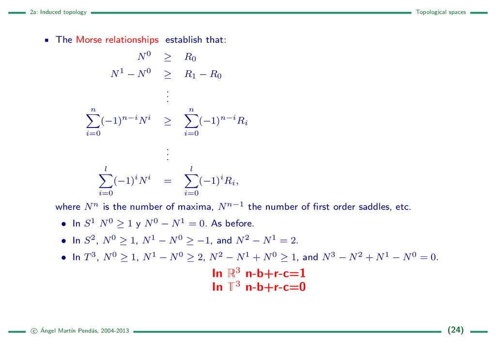
24. 2a: Induced topology Topological spaces The Morse relationships establish that: N0 R0 N1 N0 R1 R0 . . . n X i=0 ( 1)n iNi n X i=0 ( 1)n iRi . . . l X i=0 ( 1)iNi = l X i=0 ( 1)iRi, where Nn is the number of maxima, Nn 1 the number of first order saddles, etc. • In S1 N0 1 y N0 N1 = 0. As before. • In S2, N0 1, N1 N0 1, and N2 N1 = 2. • In T3, N0 1, N1 N0 2, N2 N1 + N0 1, and N3 N2 + N1 N0 = 0. In 3 n-b+r-c=1 In 3 n-b+r-c=0 c ´ Angel Mart´ ın Pend´ as, 2004-2013 (24)
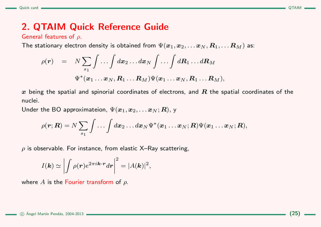
25. Quick card QTAIM 2. QTAIM Quick Reference Guide General features of ⇢. The stationary electron density is obtained from ( x1, x2, . . . xN , R1, . . . RM ) as: ⇢( r ) = N X s 1 Z . . . Z d x2 . . . d xN Z . . . Z d R1 . . . d RM ⇤( x1 . . . xN , R1 . . . RM ) ( x1 . . . xN , R1 . . . RM ), x being the spatial and spinorial coordinates of electrons, and R the spatial coordinates of the nuclei. Under the BO approximateion, ( x1, x2, . . . xN ; R ), y ⇢( r ; R ) = N X s 1 Z . . . Z d x2 . . . d xN ⇤( x1 . . . xN ; R ) ( x1 . . . xN ; R ), ⇢ is observable. For instance, from elastic X–Ray scattering, I( k ) ' Z ⇢( r )e2⇡ik·rd r 2 = |A( k )|2, where A is the Fourier transform of ⇢. c ´ Angel Mart´ ın Pend´ as, 2004-2013 (25)
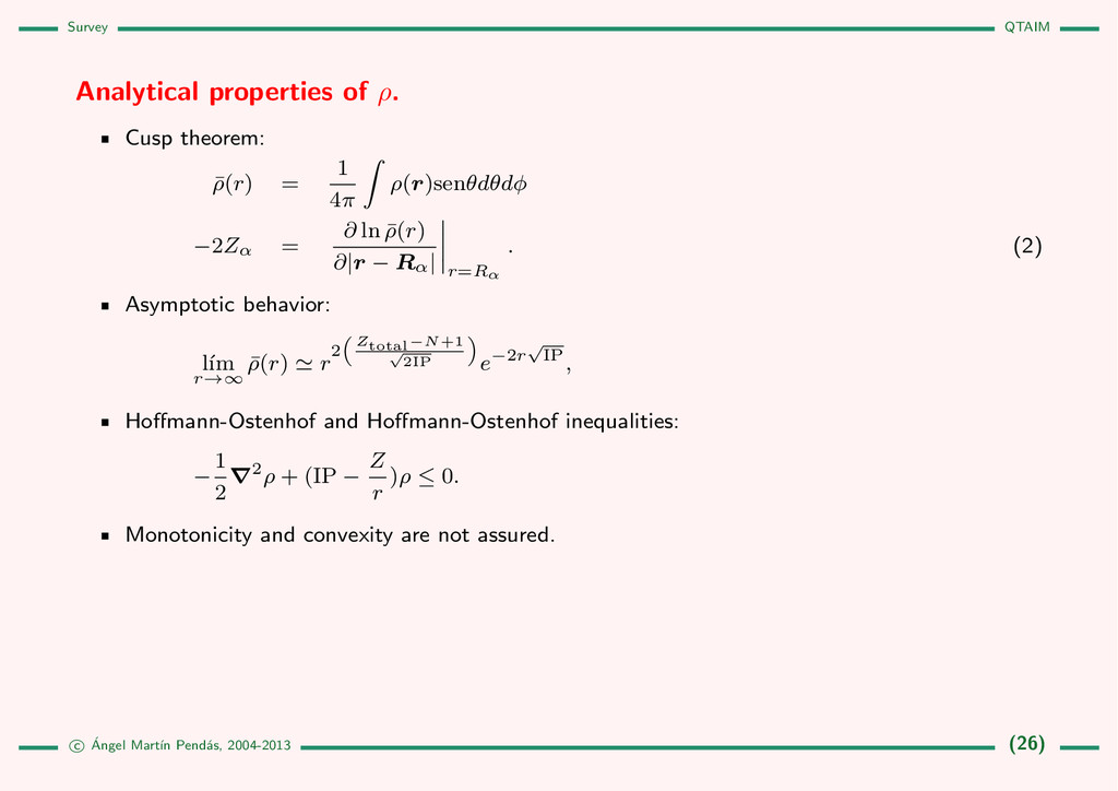
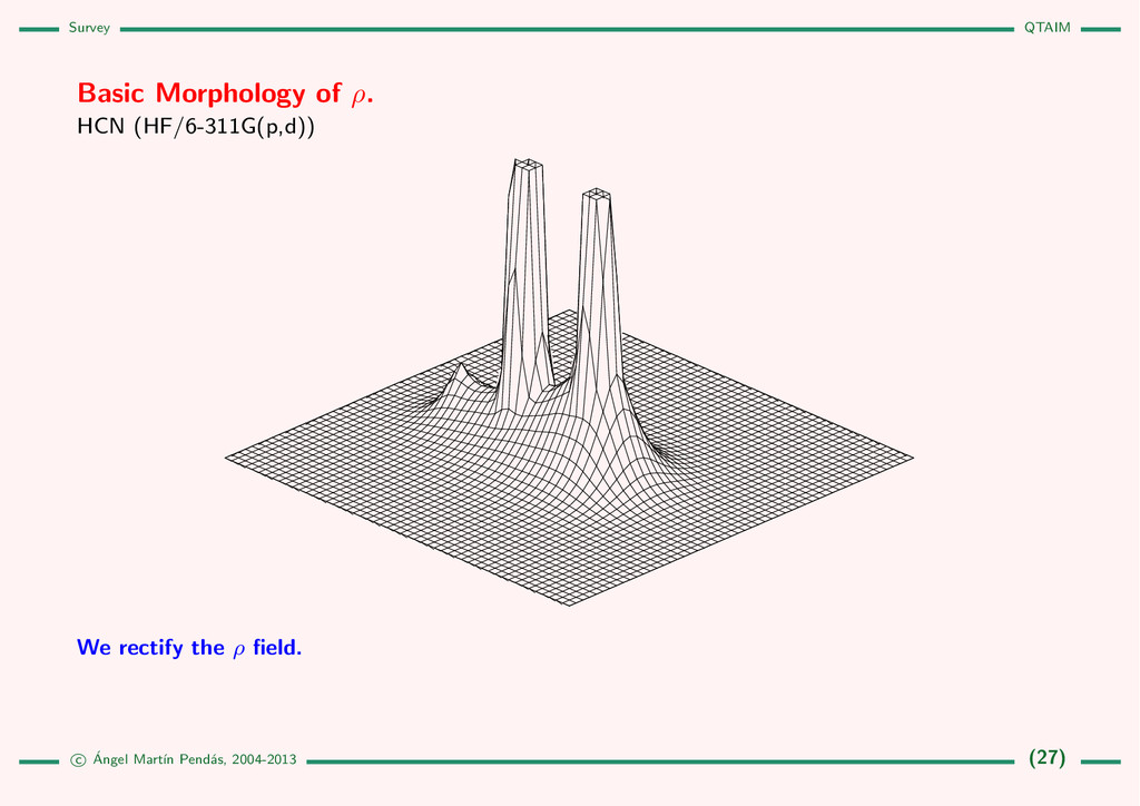
26. Survey QTAIM Analytical properties of ⇢. Cusp theorem: ¯ ⇢(r) = 1 4⇡ Z ⇢( r )sen✓d✓d 2Z↵ = @ ln ¯ ⇢(r) @| r R↵| r=R↵ . (2) Asymptotic behavior: l´ ım r!1 ¯ ⇢(r) ' r2 ⇣ Z total N +1 p 2IP ⌘ e 2r p IP, Ho↵mann-Ostenhof and Ho↵mann-Ostenhof inequalities: 1 2 r2⇢ + (IP Z r )⇢  0. Monotonicity and convexity are not assured. c ´ Angel Mart´ ın Pend´ as, 2004-2013 (26)
27. Survey QTAIM Basic Morphology of ⇢. HCN (HF/6-311G(p,d)) We rectify the ⇢ field. c ´ Angel Mart´ ın Pend´ as, 2004-2013 (27)
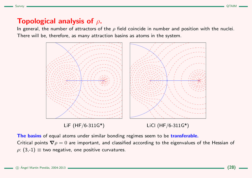
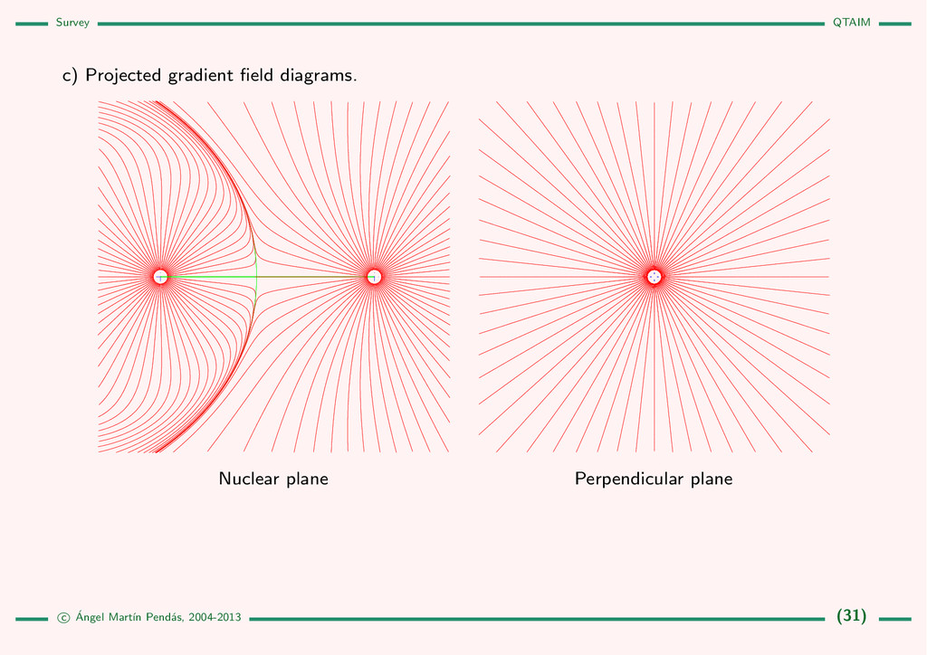
28. Survey QTAIM Topological analysis of ⇢. In general, the number of attractors of the ⇢ field coincide in number and position with the nuclei. There will be, therefore, as many attraction basins as atoms in the system. LiF (HF/6-311G*) LiCl (HF/6-311G*) The basins of equal atoms under similar bonding regimes seem to be transferable. Critical points r⇢ = 0 are important, and classified according to the eigenvalues of the Hessian of ⇢: (3,-1) ⌘ two negative, one positive curvatures. c ´ Angel Mart´ ın Pend´ as, 2004-2013 (28)
29. Survey QTAIM Usual representations. (LiH HF/TZV) a) Projected relief diagrams. Nuclear plane Perpendicular plane c ´ Angel Mart´ ın Pend´ as, 2004-2013 (29)
30. Survey QTAIM b) Projected contour diagrams. Nuclear plane Perpendicular plane c ´ Angel Mart´ ın Pend´ as, 2004-2013 (30)
31. Survey QTAIM c) Projected gradient field diagrams. Nuclear plane Perpendicular plane c ´ Angel Mart´ ın Pend´ as, 2004-2013 (31)
32. Survey QTAIM (d) Isosurfaces. ⇢ = 0.01 ⇢ = 0.02 ⇢ = 0.05 c ´ Angel Mart´ ın Pend´ as, 2004-2013 (32)
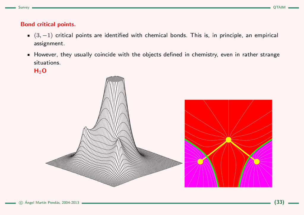
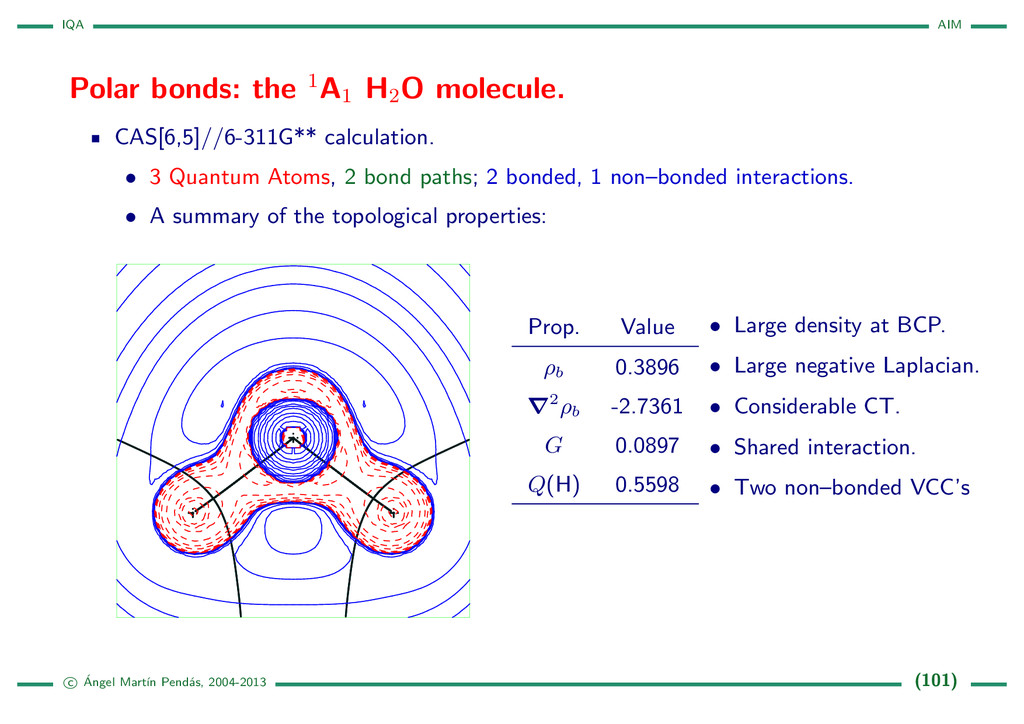
33. Survey QTAIM Bond critical points. (3, 1) critical points are identified with chemical bonds. This is, in principle, an empirical assignment. However, they usually coincide with the objects defined in chemistry, even in rather strange situations. H2O c ´ Angel Mart´ ın Pend´ as, 2004-2013 (33)