Measuring the Undetectable

Galaxy coffee at MPIA. August 2011.

Transcript

2. Dan Foreman-Mackey (NYU) Aug. 18, 2011 Galaxy Coffee Measuring the Undetectable Calibration in the time domain and 2.0
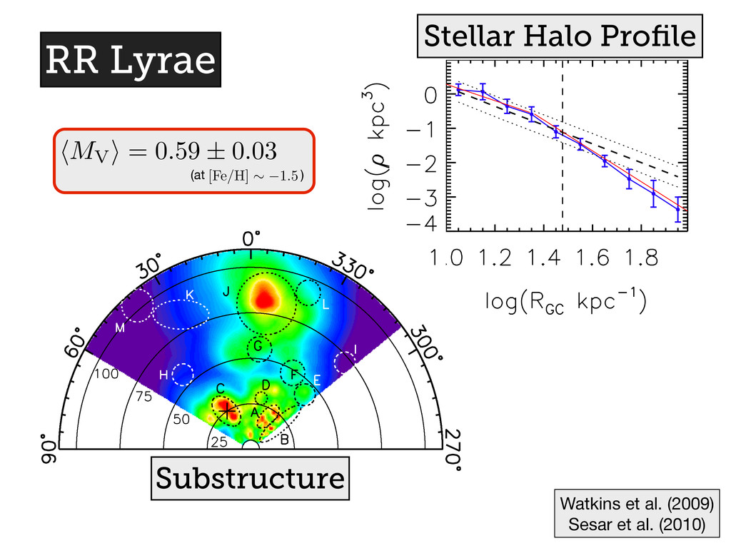
3. RR Lyrae Figure 14. Radial number density profiles for four regions in R.A.: 30◦ < R.A. < 60◦ (top left), 0◦ < R.A. < 30◦ (top right), 340◦ < R.A. < 0◦ (bottom left), and 310◦ < R.A. < 340◦ (bottom right). The bottom left panel contains the Pisces overdensity at RGC ∼ 80 kpc (log(RGC) ∼ 1.9). The symbols show the observed median number density and the rms scatter around the median value for pixels shown in Figure 11 (top). The dashed line shows the number density predicted from the smooth model (log(ρRR model ), Equation (16)), and the dotted lines show the ±0.3 dex envelope (a factor of 2) around the predicted values which corresponds to the sample Poisson noise determined from model-based number density maps. The solid line shows the prediction from Watkins et al. (2009). The ρRR in Equation (16) was increased by 33% to 5.6 kpc−3 to match Figure 14. Radial number density profiles for fo R.A. < 60◦ (top left), 0◦ < R.A. < 30◦ (top right), left), and 310◦ < R.A. < 340◦ (bottom right). The b Pisces overdensity at RGC ∼ 80 kpc (log(RGC) ∼ 1 observed median number density and the rms scatt for pixels shown in Figure 11 (top). The dashed lin predicted from the smooth model (log(ρRR model ), Equ lines show the ±0.3 dex envelope (a factor of 2) a which corresponds to the sample Poisson noise det number density maps. The solid line shows the pre (2009). The ρRR in Equation (16) was increased by SESAR ET AL. S07 Labela A B C D E F G H I Watkins et al. (2009) Sesar et al. (2010) Substructure Stellar Halo Profile hMV i = 0.59 ± 0.03 [Fe/H] ⇠ 1.5 (at )
7. Zero Points
8. ~Time ~Time Zero Points
9. cas.sdss.org
10. cas.sdss.org
11. cas.sdss.org
12. p(X|⇥) = N Y ↵ =1 [(1 P var )p const (X↵ |⇥) + P var p var (X↵ |⇥)] Our Calibration Model DFM, Hogg, et al. (in prep)
13. p(X|⇥) = N Y ↵ =1 [(1 P var )p const (X↵ |⇥) + P var p var (X↵ |⇥)] Stars Our Calibration Model DFM, Hogg, et al. (in prep)
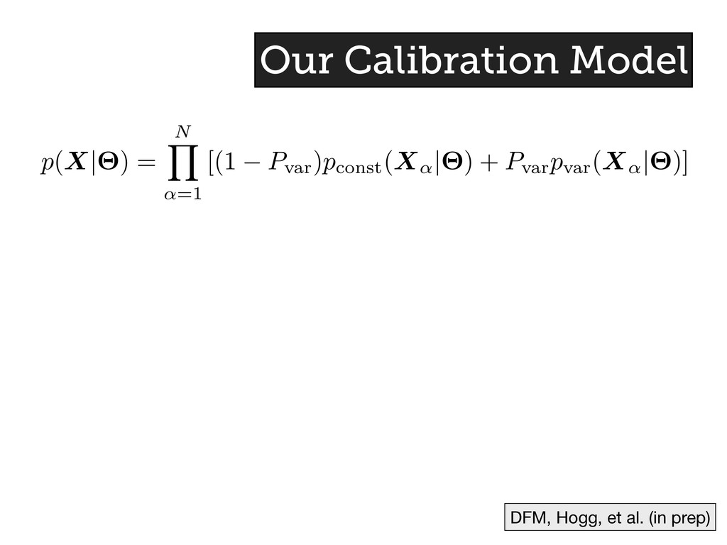
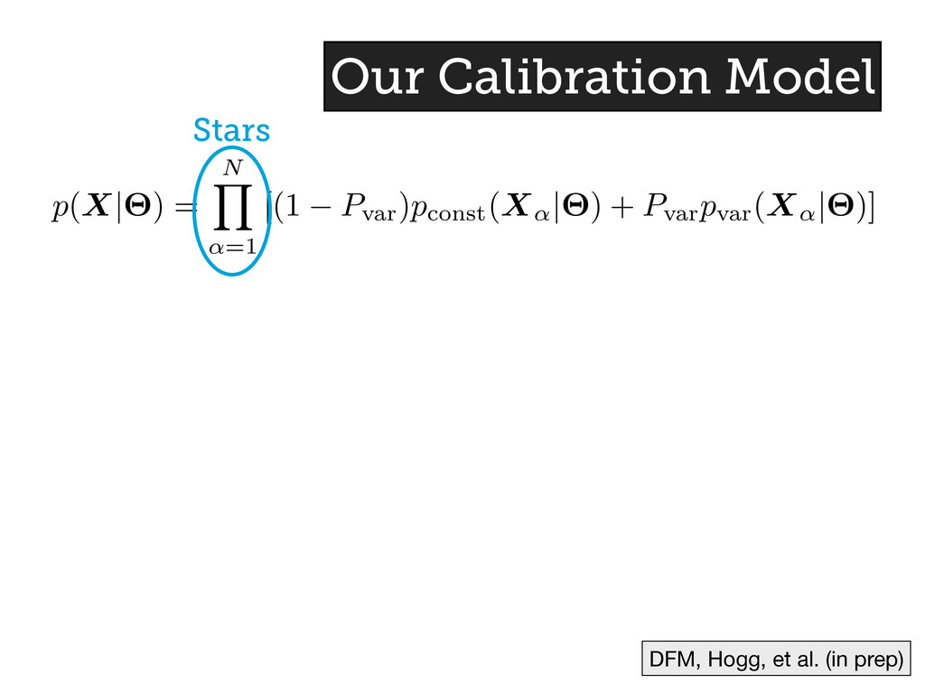
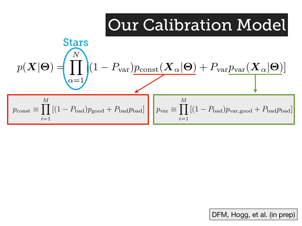
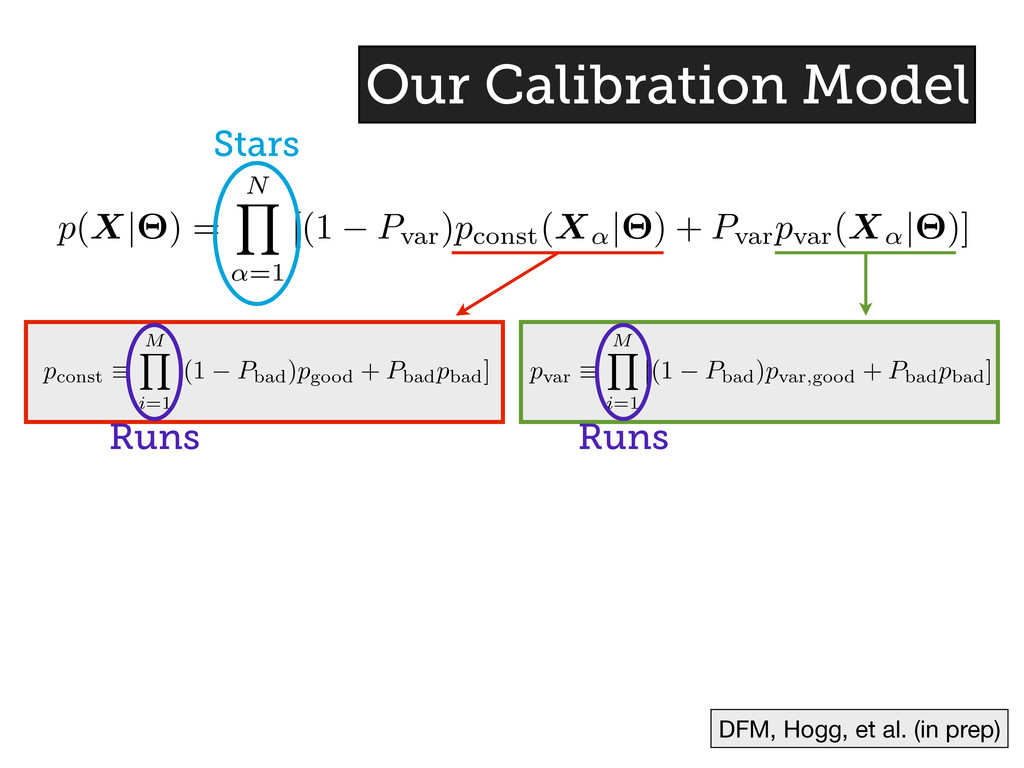
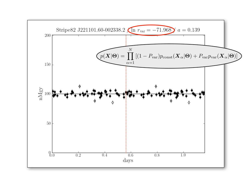
14. p(X|⇥) = N Y ↵ =1 [(1 P var )p const (X↵ |⇥) + P var p var (X↵ |⇥)] p const ⌘ M Y i =1 [(1 P bad )p good + P bad p bad ] p var ⌘ M Y i =1 [(1 P bad )p var , good + P bad p bad ] Stars Our Calibration Model DFM, Hogg, et al. (in prep)
15. p(X|⇥) = N Y ↵ =1 [(1 P var )p const (X↵ |⇥) + P var p var (X↵ |⇥)] p const ⌘ M Y i =1 [(1 P bad )p good + P bad p bad ] p var ⌘ M Y i =1 [(1 P bad )p var , good + P bad p bad ] Stars Runs Runs Our Calibration Model DFM, Hogg, et al. (in prep)
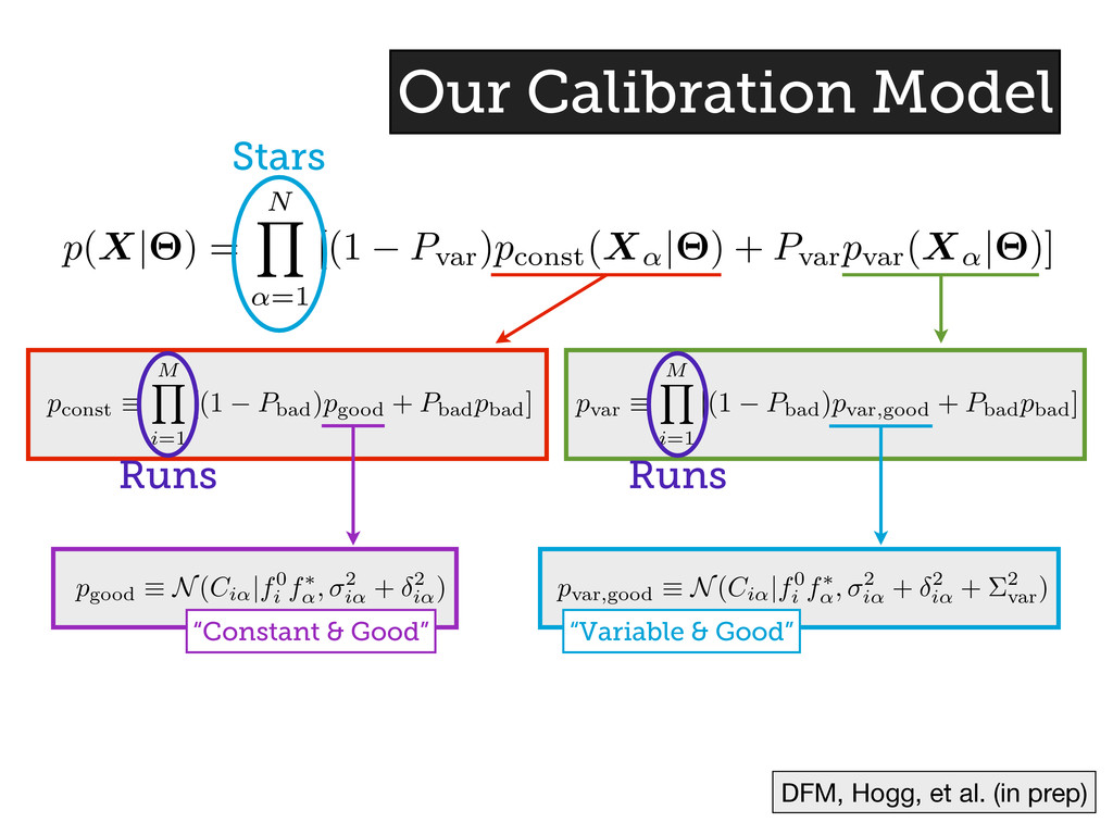
16. p(X|⇥) = N Y ↵ =1 [(1 P var )p const (X↵ |⇥) + P var p var (X↵ |⇥)] p const ⌘ M Y i =1 [(1 P bad )p good + P bad p bad ] p var ⌘ M Y i =1 [(1 P bad )p var , good + P bad p bad ] Stars Runs Runs Our Calibration Model p good ⌘ N(Ci↵ |f0 i f⇤ ↵ , 2 i↵ + 2 i↵ ) “Constant & Good” p var , good ⌘ N(Ci↵ |f0 i f⇤ ↵ , 2 i↵ + 2 i↵ + ⌃2 var ) “Variable & Good” DFM, Hogg, et al. (in prep)
17. p(X|⇥) = N Y ↵ =1 [(1 P var )p const (X↵ |⇥) + P var p var (X↵ |⇥)] p const ⌘ M Y i =1 [(1 P bad )p good + P bad p bad ] p var ⌘ M Y i =1 [(1 P bad )p var , good + P bad p bad ] Stars Runs Runs Our Calibration Model p good ⌘ N(Ci↵ |f0 i f⇤ ↵ , 2 i↵ + 2 i↵ ) “Constant & Good” p var , good ⌘ N(Ci↵ |f0 i f⇤ ↵ , 2 i↵ + 2 i↵ + ⌃2 var ) “Variable & Good” pbad ⌘ N(Ci↵ |f0 i f⇤ ↵ , 2 i↵ + 2 i↵ + ⌃2 bad ) “Bad” DFM, Hogg, et al. (in prep)
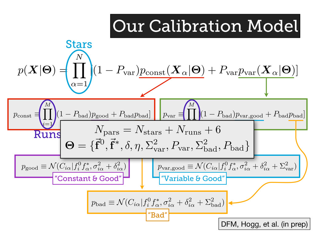
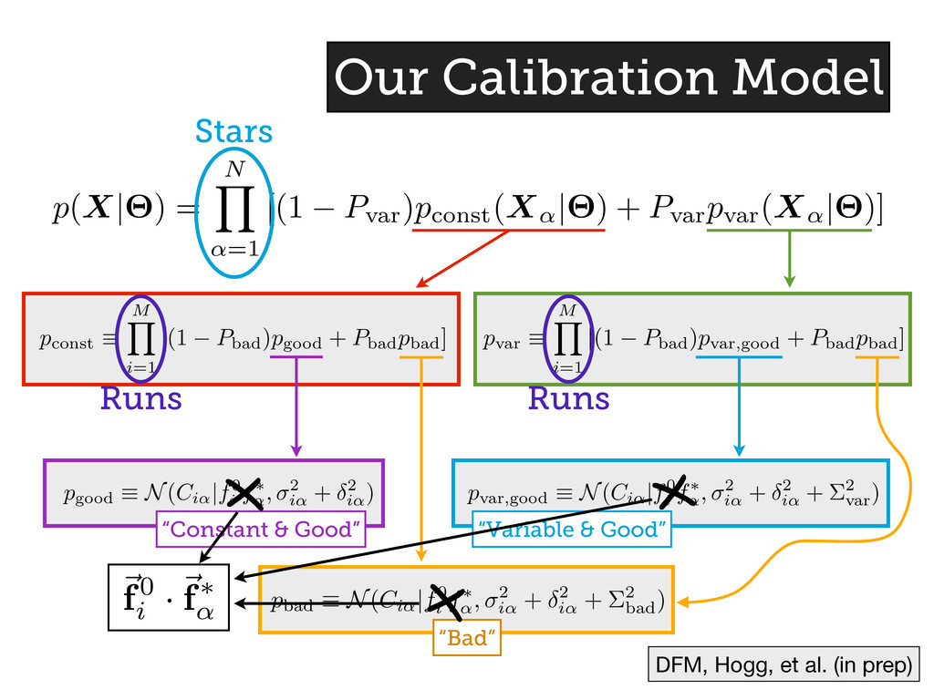
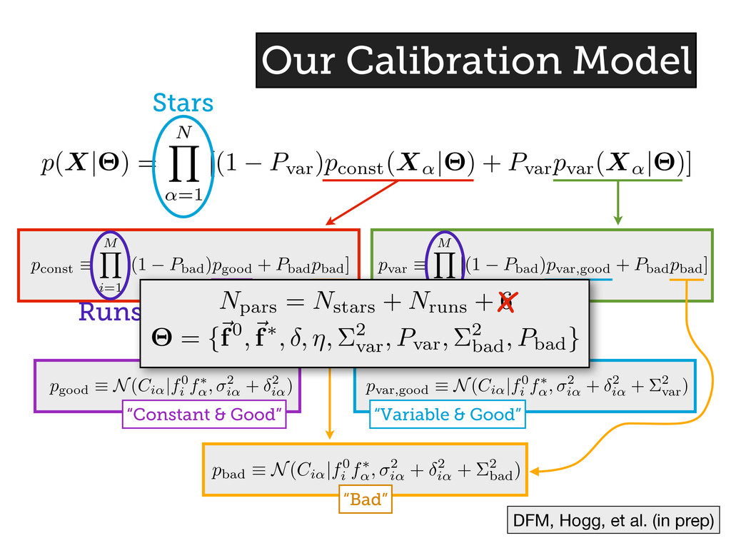
18. p(X|⇥) = N Y ↵ =1 [(1 P var )p const (X↵ |⇥) + P var p var (X↵ |⇥)] p const ⌘ M Y i =1 [(1 P bad )p good + P bad p bad ] p var ⌘ M Y i =1 [(1 P bad )p var , good + P bad p bad ] Stars Runs Runs Our Calibration Model p good ⌘ N(Ci↵ |f0 i f⇤ ↵ , 2 i↵ + 2 i↵ ) “Constant & Good” p var , good ⌘ N(Ci↵ |f0 i f⇤ ↵ , 2 i↵ + 2 i↵ + ⌃2 var ) “Variable & Good” pbad ⌘ N(Ci↵ |f0 i f⇤ ↵ , 2 i↵ + 2 i↵ + ⌃2 bad ) “Bad” DFM, Hogg, et al. (in prep) Npars = Nstars + Nruns + 6 ⇥ = {~ f0,~ f⇤, , ⌘, ⌃2 var , Pvar, ⌃2 bad , Pbad }
19. p(X|⇥) = N Y ↵ =1 [(1 P var )p const (X↵ |⇥) + P var p var (X↵ |⇥)] p const ⌘ M Y i =1 [(1 P bad )p good + P bad p bad ] p var ⌘ M Y i =1 [(1 P bad )p var , good + P bad p bad ] Stars Runs Runs Our Calibration Model p good ⌘ N(Ci↵ |f0 i f⇤ ↵ , 2 i↵ + 2 i↵ ) “Constant & Good” p var , good ⌘ N(Ci↵ |f0 i f⇤ ↵ , 2 i↵ + 2 i↵ + ⌃2 var ) “Variable & Good” pbad ⌘ N(Ci↵ |f0 i f⇤ ↵ , 2 i↵ + 2 i↵ + ⌃2 bad ) “Bad” DFM, Hogg, et al. (in prep) Npars = Nstars + Nruns + 6 ⇥ = {~ f0,~ f⇤, , ⌘, ⌃2 var , Pvar, ⌃2 bad , Pbad } X
22. p(X|⇥) = N Y ↵ =1 [(1 P var )p const (X↵ |⇥) + P var p var (X↵ |⇥)]
23. Known RR Lyrae f⇤ ( t ) = A0 + N X n=1 [ An sin( !t ) + Bn cos( !t )]
24. A new candidate? ??
25. p(X|⇥) = N Y ↵ =1 [(1 P var )p const (X↵ |⇥) + P var p var (X↵ |⇥)] p const ⌘ M Y i =1 [(1 P bad )p good + P bad p bad ] p var ⌘ M Y i =1 [(1 P bad )p var , good + P bad p bad ] Stars Runs Runs Our Calibration Model p good ⌘ N(Ci↵ |f0 i f⇤ ↵ , 2 i↵ + 2 i↵ ) “Constant & Good” p var , good ⌘ N(Ci↵ |f0 i f⇤ ↵ , 2 i↵ + 2 i↵ + ⌃2 var ) “Variable & Good” pbad ⌘ N(Ci↵ |f0 i f⇤ ↵ , 2 i↵ + 2 i↵ + ⌃2 bad ) “Bad” DFM, Hogg, et al. (in prep)
26. p(X|⇥) = N Y ↵ =1 [(1 P var )p const (X↵ |⇥) + P var p var (X↵ |⇥)] p const ⌘ M Y i =1 [(1 P bad )p good + P bad p bad ] p var ⌘ M Y i =1 [(1 P bad )p var , good + P bad p bad ] Stars Runs Runs Our Calibration Model p good ⌘ N(Ci↵ |f0 i f⇤ ↵ , 2 i↵ + 2 i↵ ) “Constant & Good” p var , good ⌘ N(Ci↵ |f0 i f⇤ ↵ , 2 i↵ + 2 i↵ + ⌃2 var ) “Variable & Good” pbad ⌘ N(Ci↵ |f0 i f⇤ ↵ , 2 i↵ + 2 i↵ + ⌃2 bad ) “Bad” DFM, Hogg, et al. (in prep) ~ f0 i ·~ f⇤ ↵ X X X
27. Thanks! Check out: dfm.github.com For info about my projects and a sweet MCMC sampler written in Python!