Probabilistic modeling and Inference in Astronomy

Guest lecture for "Inference and Representation" at NYU

Transcript

1. Probabilistic modeling and Inference in Astronomy Dan Foreman-Mackey Sagan Fellow, University of Washington github.com/dfm // @exoplaneteer // dfm.io
2. Dan Foreman-Mackey Sagan Fellow, University of Washington github.com/dfm // @exoplaneteer // dfm.io
3. I study astronomy. Photo credit NASA Ames/SETI Institute/JPL-Caltech
4. I study astronomy. Photo credit NASA Ames/SETI Institute/JPL-Caltech this isn't what my data look like
5. Why Astronomy? simple but interesting physical models precise open-access data observational only
6. Why Astronomy? simple but interesting physical models precise open-access data observational only no chance of financial gain ever
7. ex·o·plan·et ˈeksōˌplanət/ noun. a planet that orbits a star outside the solar system. Credit Google
8. How do we find & study exoplanets?
9. transit radial velocity direct imaging microlensing timing astrometry 1281 616 45 32 20 0 Data from Open Exoplanet Catalogue
10. Data from Open Exoplanet Catalogue 2000 2005 2010 2015 year of discovery 0 200 400 600 800 1000 number of exoplanets transit RV microlensing direct imaging timing
11. Data from Open Exoplanet Catalogue 2000 2005 2010 2015 year of discovery 0 200 400 600 800 1000 number of exoplanets transit RV microlensing direct imaging timing first public data release from Kepler
12. the transit method
13. Credit NASA/European Space Agency
14. Credit NASA/European Space Agency Jupiter
15. Credit NASA/European Space Agency Jupiter Earth
16. that's not what most stars look like!
18. 1.0 0.5 0.0 0.5 1.0 time since transit [days] 100 50 0 relative brightness [ppm]
19. everything is against us!
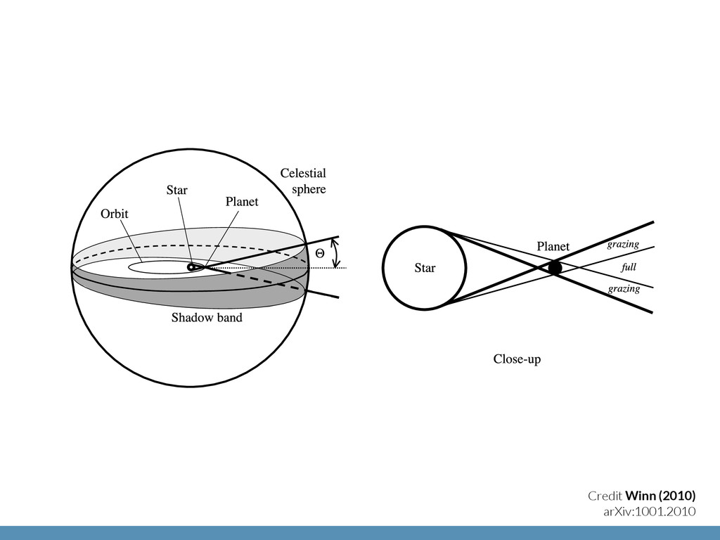
20. Fig. 3.— Calculation of the transit probability. Left.—Transits are visible by observers within the penumbra of the planet, a cone with opening angle Θ with sin Θ = (R⋆ +Rp )/r, where r is the instantaneous star-planet distance. Right.—Close-up showing the penumbra (thick lines) as well as the antumbra (thin lines) within which the transits are full, as opposed to grazing. are tangent at four contact times tI –tIV , illustrated in Fig- ure 2. (In a grazing eclipse, second and third contact do not occur.) The total duration is Ttot = tIV − tI , the full duration is Tfull = tIII − tII , the ingress duration is ingress and egress. In practice the difference is slight; to leading order in R⋆/a and e, τe − τi ∼ e cosω R⋆ 3 1 − b2 3/2 , (17) Credit Winn (2010) arXiv:1001.2010
21. need to look at the right place at the right time and measure extremely precise photometry
22. Credit NASA Kepler
23. Credit NASA
24. Credit Carter Roberts
25. Credit NASA
26. Kepler-32
27. Kepler-32
28. Kepler-32
29. Kepler-32
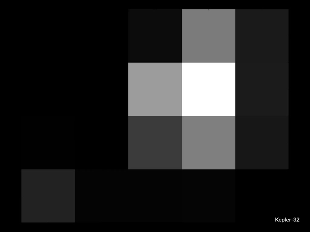
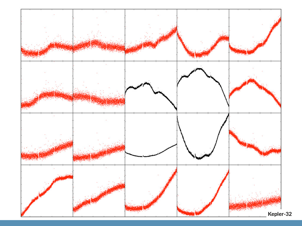
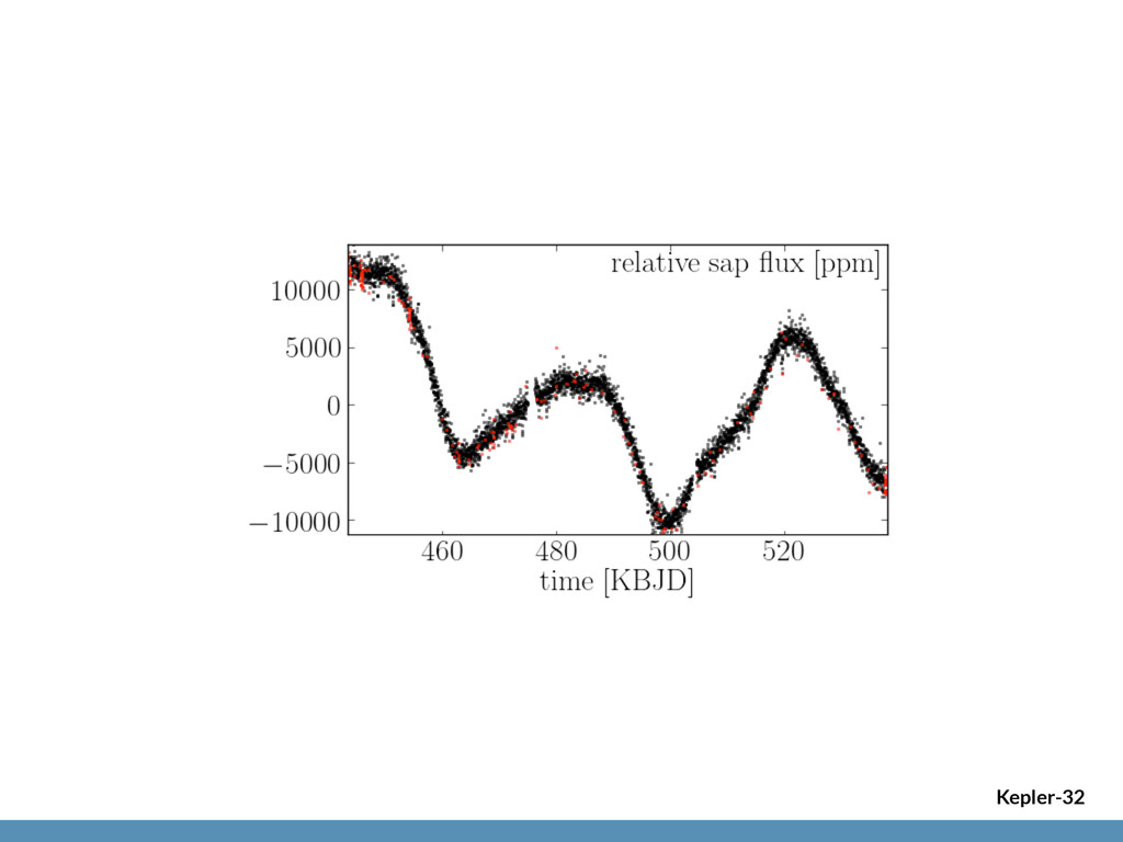
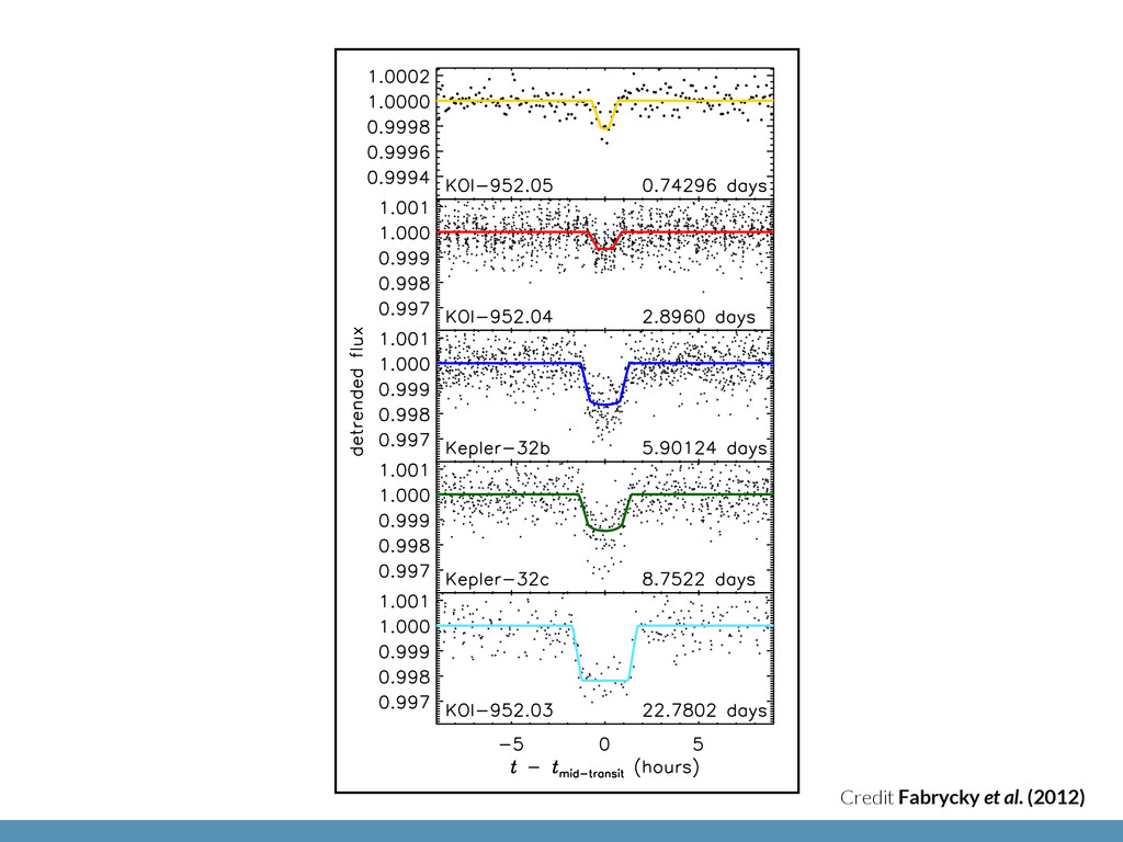
30. Credit Fabrycky et al. (2012) 12 Fabrycky et al. Figure 16. Kepler-31 phase curves, in the style of figure 3. For the small inner candidate KOI-952.05, the phase is with respect to terest. The Kepler Follow-up spectra of Kepler-32: one sp servatory and one from Keck are weak due to the faintness cross correlation function be and available models is max ∼ 3900 K and ∼ 3600 K, atmospheric parameters are star is cooler than the library able. Both spectra are con sification as a cool dwarf ( [M/H]=0.172). We conserva Teff and log g with uncertain a [M/H] of 0± 0.4 based on t By comparing to the Yonse values for the stellar mass ( (0.53 ± 0.04R⊙ ) that are sli the KIC. We estimate a lum and an age of ≤ 9Gyr. Muirhead et al. (2011) h resolution IR spectrum of K a stellar Teff = 3726+73 −67 , [Fe ing their data via Padova m they inferred a considerably l We encourage further detail properties, as these have con directly affect the sizes and The probability of a star u being the actual host is only ity of a physical companion h This latter number is relative all the transit depths are sma be much larger planets hoste ically diluted. This opens up
31. 101 102 orbital period [days] 100 101 planet radius [R ] Data from NASA Exoplanet Archive
32. that looks pretty good…
33. 101 102 orbital period [days] 100 101 planet radius [R ] Data from NASA Exoplanet Archive
34. 101 102 orbital period [days] 100 101 planet radius [R ] Data from NASA Exoplanet Archive
35. 100 101 102 103 104 105 orbital period [days] 100 101 planet radius [R ] Data from NASA Exoplanet Archive
36. May 2013 The Kepler Mission goes up in flames * not exactly
37. Credit NASA Kepler RIP
38. cbna Flickr user Aamir Choudhry introducing: K2
39. Credit NASA K2
42. 4000 2000 0 2000 4000 raw: 301 ppm EPIC 201374602; Kp = 11.5 mag 10 20 30 40 50 60 70 80 time [BJD - 2456808] 400 0 400 residuals: 35 ppm relative brightness [ppm] 4000 2000 0 2000 4000 raw: 301 ppm EPIC 201374602; Kp = 11.5 mag 10 20 30 40 50 60 70 80 time [BJD - 2456808] 400 0 400 residuals: 35 ppm relative brightness [ppm]
43. 7.2 7.4 7.6 x [pix] 10 20 30 40 50 60 70 80 time [BJD - 2456808] 9.05 9.10 9.15 9.20 y [pix]
44. Can we find planets using K2?
45. Anatomy of a transit signal + + + = planet star space craft detector signal
46. Designing the probabilistic model n Pn xn K Sn stars: n = 1, · · · , N n Pn xn K Sn planet star space craft detector
47. Designing the probabilistic model planet: star: noise: space craft: physics and geometry continuous in time → GP CCD, photon noise → Poisson ?? representation:
48. The planet orbit model cba Wikipedia user Gonfer Kepler's Laws of Planetary Motion
49. The planet orbit model cba Wikipedia user Gonfer Kepler's Laws of Planetary Motion
50. TRANSIT LIGHT CURVES Vol. 580 mb darkening. The star is seen edge-on, with the observer off the top of the page. The star has radius , and v is defined as the r∗ d the normal to the stellar surface, while . (b) Transit geometry from the perspective of the observer. m p cos v 3. NONLINEAR LIMB DARKENING s a star to be more centrally peaked in brightness compared to a uniform source. This leads to more ng eclipse and creates curvature in the trough. Thus, including limb darkening is important for computing Reference Mandel & Agol (2002); arXiv:astro-ph/0210099 The planet transit model
51. TRANSIT LIGHT CURVES Vol. 580 mb darkening. The star is seen edge-on, with the observer off the top of the page. The star has radius , and v is defined as the r∗ d the normal to the stellar surface, while . (b) Transit geometry from the perspective of the observer. m p cos v 3. NONLINEAR LIMB DARKENING s a star to be more centrally peaked in brightness compared to a uniform source. This leads to more ng eclipse and creates curvature in the trough. Thus, including limb darkening is important for computing Reference Mandel & Agol (2002); arXiv:astro-ph/0210099 The planet transit model
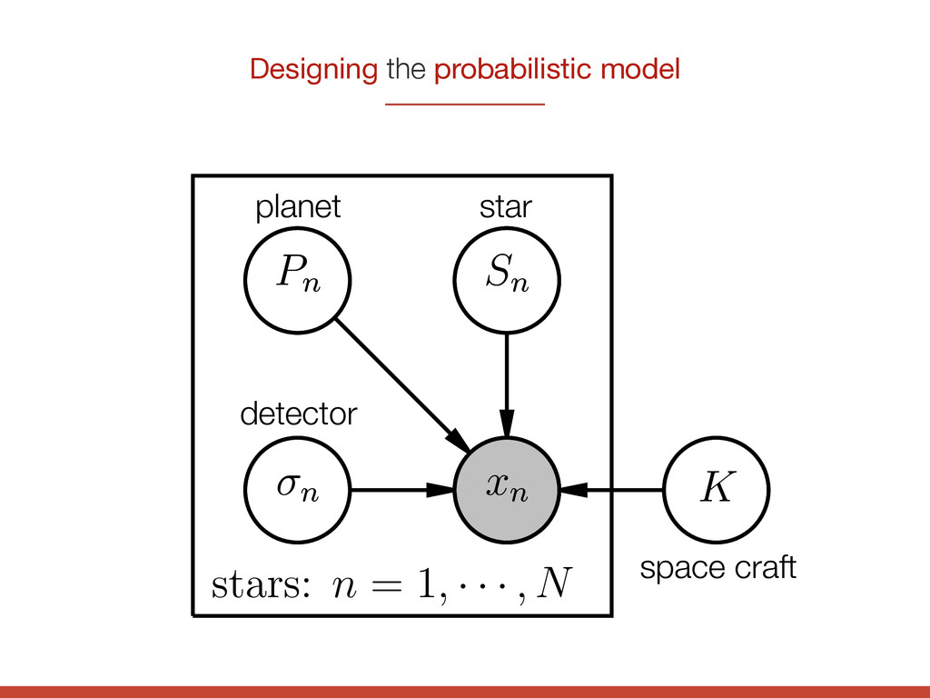
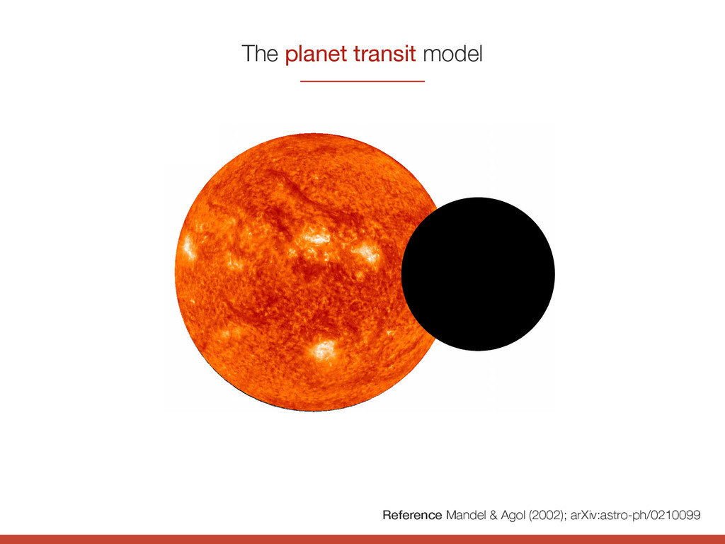
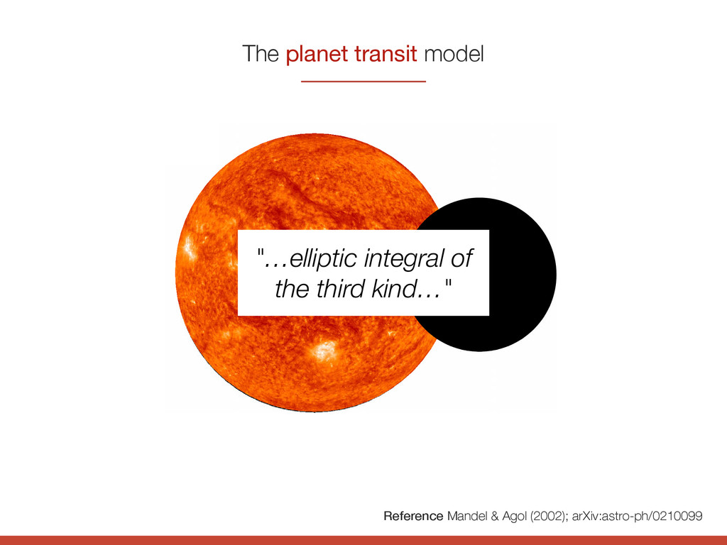
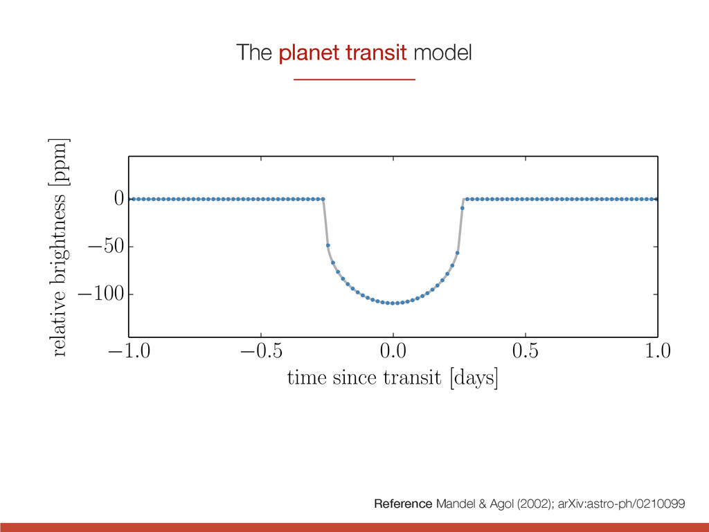
52. TRANSIT LIGHT CURVES Vol. 580 mb darkening. The star is seen edge-on, with the observer off the top of the page. The star has radius , and v is defined as the r∗ d the normal to the stellar surface, while . (b) Transit geometry from the perspective of the observer. m p cos v 3. NONLINEAR LIMB DARKENING s a star to be more centrally peaked in brightness compared to a uniform source. This leads to more ng eclipse and creates curvature in the trough. Thus, including limb darkening is important for computing Reference Mandel & Agol (2002); arXiv:astro-ph/0210099 The planet transit model "…elliptic integral of the third kind…"
53. TRANSIT LIGHT CURVES Vol. 580 mb darkening. The star is seen edge-on, with the observer off the top of the page. The star has radius , and v is defined as the r∗ d the normal to the stellar surface, while . (b) Transit geometry from the perspective of the observer. m p cos v 3. NONLINEAR LIMB DARKENING s a star to be more centrally peaked in brightness compared to a uniform source. This leads to more ng eclipse and creates curvature in the trough. Thus, including limb darkening is important for computing Reference Mandel & Agol (2002); arXiv:astro-ph/0210099 The planet transit model "…elliptic integral of the third kind…" 1.0 0.5 0.0 0.5 1.0 time since transit [days] 100 50 0 relative brightness [ppm]
54. Designing the probabilistic model planet: star: noise: space craft: physics and geometry continuous in time → GP CCD, photon noise → Poisson ?? representation:
55. The stellar variability model
56. The stellar variability model y ⇠ N(f✓ (t), K↵(t)) Gaussian Mean Covariance
57. 0 1 2 3 4 5 x 6 4 2 0 2 4 6 y y ⇠ N (f✓ (t), K↵(t))
58. 0 1 2 3 4 5 x 6 4 2 0 2 4 6 y y ⇠ N (f✓ (t), K↵(t))
59. 0 1 2 3 4 5 x 6 4 2 0 2 4 6 y y ⇠ N (f✓ (t), K↵(t))
60. 0 1 2 3 4 5 x 6 4 2 0 2 4 6 y y ⇠ N (f✓ (t), K↵(t))
61. The stellar variability model
62. Designing the probabilistic model planet: star: noise: space craft: physics and geometry continuous in time → GP CCD, photon noise → Poisson ?? representation:
63. Credit NASA The noise model
64. Designing the probabilistic model planet: star: noise: space craft: physics and geometry continuous in time → GP CCD, photon noise → Poisson ?? representation:
65. Designing the probabilistic model n Pn xn K Sn stars: n = 1, · · · , N n Pn xn K Sn
66. stars: n = 1, · · · , N n xn K Designing the probabilistic model simple space craft assumption:
67. 4000 2000 0 2000 4000 raw: 301 ppm EPIC 201374602; Kp = 11.5 mag 10 20 30 40 50 60 70 80 time [BJD - 2456808] 400 0 400 residuals: 35 ppm relative brightness [ppm] 4000 2000 0 2000 4000 raw: 301 ppm EPIC 201374602; Kp = 11.5 mag 10 20 30 40 50 60 70 80 time [BJD - 2456808] 400 0 400 residuals: 35 ppm relative brightness [ppm]
68. 20 40 60 80 time [BJD - 2456808]
69. 60 62 64 66 68 70 time [BJD - 2456808]
70. 4000 2000 0 2000 4000 raw: 301 ppm EPIC 201374602; Kp = 11.5 mag 10 20 30 40 50 60 70 80 time [BJD - 2456808] 400 0 400 residuals: 35 ppm relative brightness [ppm]
71. Designing the probabilistic model planet: star: noise: space craft: physics and geometry continuous in time → GP CCD, photon noise → Poisson data-driven linear model representation:
72. Designing the probabilistic model n Pn xn K Sn stars: n = 1, · · · , N n Pn xn K Sn
73. n Pn xn K Sn Designing the probabilistic model
74. 2 0 2 4 (a) raw 4 2 0 (b) 10 ELCs depth: 3.2 ppt 4 2 0 (c) 150 ELCs depth: 2.7 ppt 63 64 65 66 67 time [BJD - 2456808] 4 2 0 (d) conditional depth: 3.7 ppt relative brightness [ppt]
75. Can we find planets using K2?
76. Yes.
77. stars days of data planet candidates confirmed planets 21,703 80 36 18 K2 Campaign 1 exoplanet discoveries Published: Foreman-Mackey, Montet, Hogg, et al. (arXiv:1502.04715) Montet, Morton, Foreman-Mackey, et al. (arXiv:1503.07866) Schölkopf, Hogg, Wang, Foreman-Mackey, et al. (arXiv:1505.03036)
78. XKCD/1555
79. XKCD/1555
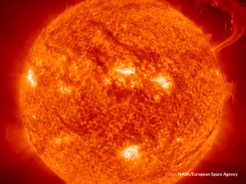
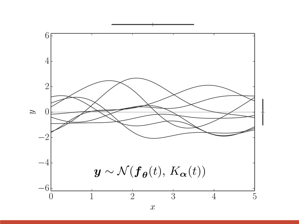
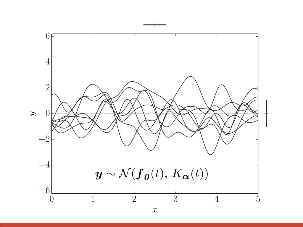
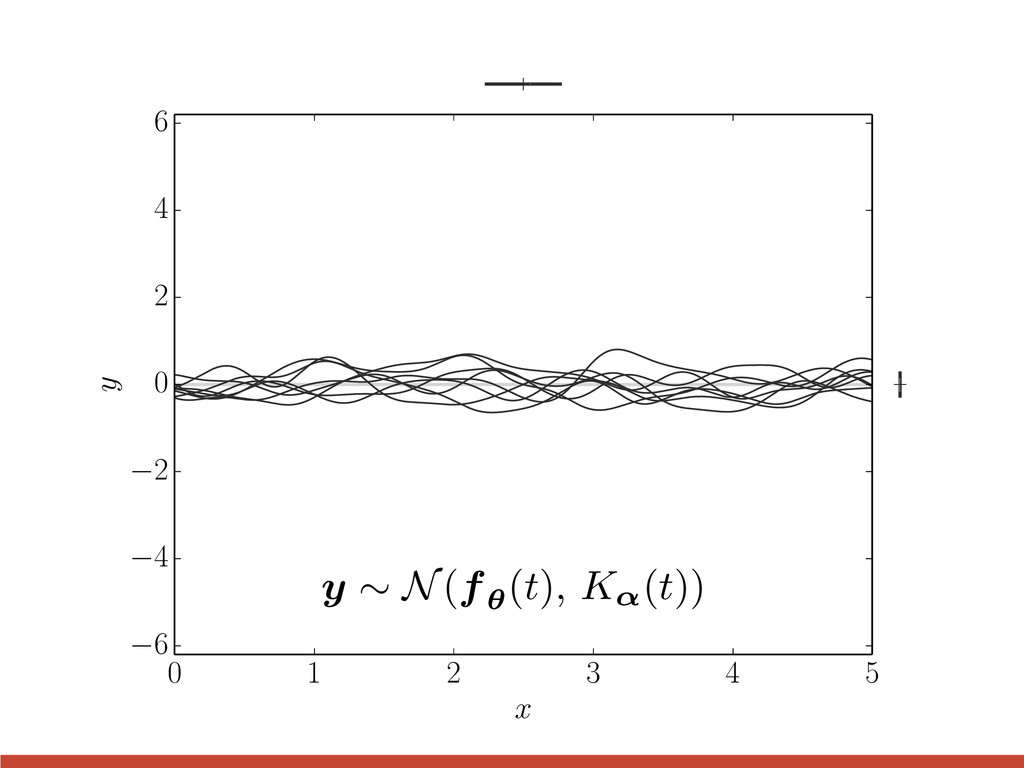
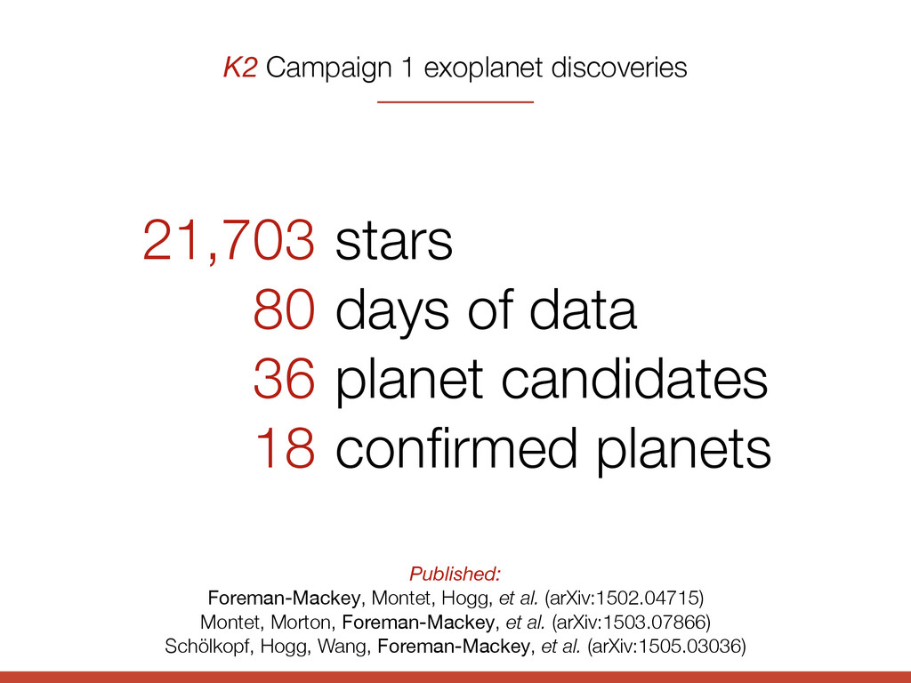
80. Foreman-Mackey, Montet, Hogg, et al. (arXiv:1502.04715) Montet, Morton, Foreman-Mackey, et al. (arXiv:1503.07866) Schölkopf, Hogg, Wang, Foreman-Mackey, et al. (arXiv:1505.03036) Probabilistic modeling—combining physical and data-driven models—enables the discovery of new planets using open data and open source software