FISH 6000: Week 3 - Simple linear regression

Linear Regression

Transcript

1. Chapter 3: Simple linear regression CatchRate ~ Poisson (μ ij ) E(CatchRate) = μ ij Log(μ ij ) = GearType ij + Temperature ij + FleetDeployment i FleetDeployment i ~ N(0, σ2) Using lme4: m <- glmer(CatchRate ~ GearType + Temperature + (1 | FleetDeployment), family = poisson) FISH 6003 FISH 6003: Statistics and Study Design for Fisheries Brett Favaro 2017 This work is licensed under a Creative Commons Attribution 4.0 International License
2. Land Acknowledgment We would like to respectfully acknowledge the territory in which we gather as the ancestral homelands of the Beothuk, and the island of Newfoundland as the ancestral homelands of the Mi’kmaq and Beothuk. We would also like to recognize the Inuit of Nunatsiavut and NunatuKavut and the Innu of Nitassinan, and their ancestors, as the original people of Labrador. We strive for respectful partnerships with all the peoples of this province as we search for collective healing and true reconciliation and honour this beautiful land together. http://www.mun.ca/aboriginal_affairs/
3. This week: • Simple (bivariate) linear regression
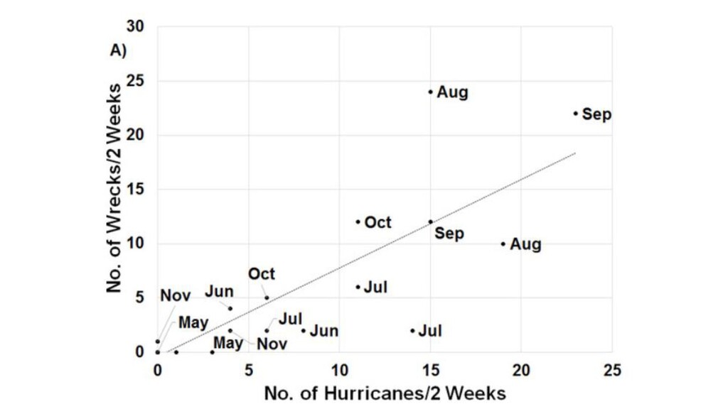
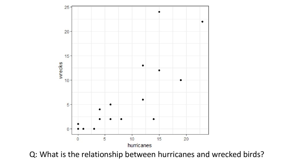
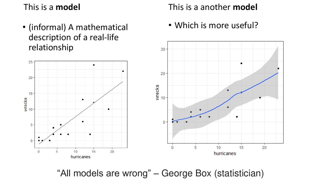
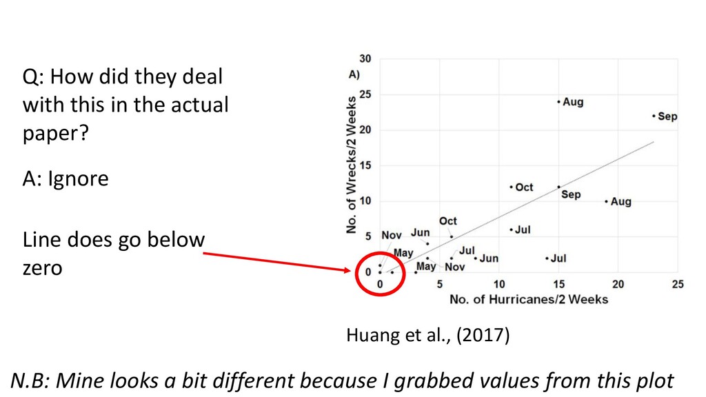
4. https://peerj.com/articles/3287/ We combined telemetry data on Onychoprion fuscatus (sooty terns) with a long-term capture- mark-recapture dataset from the Dry Tortugas National Park to map the movements at sea for this species, calculate estimates of mortality, and investigate the impact of hurricanes on a migratory seabird. … Indices of hurricane strength and occurrence are positively correlated with annual mortality and indices of numbers of wrecked birds.
6. Q: What is the relationship between hurricanes and wrecked birds?
7. Draw a line through the points Goal: Minimize the distance between the line and each point Sometimes called “line of best fit” Important: This line must not extend beyond the x range
8. What is the line really illustrating? R calculates a ‘predicted value’ at each value of X, and connects as a line This is our modelled relationship These are our predicted values from the model
9. This is a model • (informal) A mathematical description of a real-life relationship This is a another model “All models are wrong” – George Box (statistician) • Which is more useful?
10. Residuals: Distance between the observed values and predicted values The line is fit so as to minimize residuals
11. This demonstrates why Y outliers are so impactful! Technically… to minimize the sum of squared residuals
12. Y = mX + B Y = Y m = slope X = X B = intercept Y = 1(X) + 0 Y = 1(X) + 0.5 Y = 2(X) + 0 Y = 2(X) + 0.5 Recall: How to draw a line
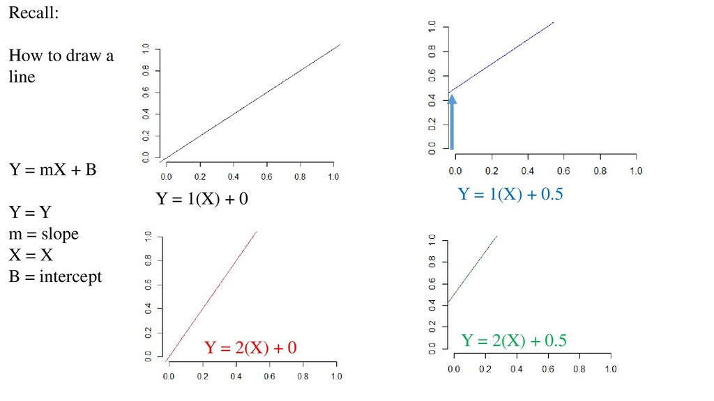
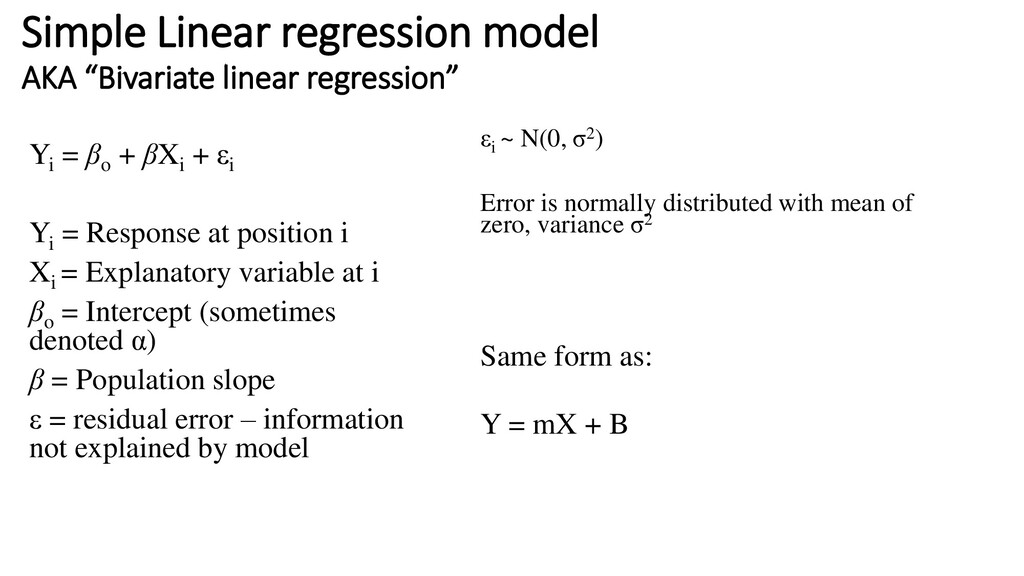
13. Simple Linear regression model Yi = βo + βXi + εi Yi = Response at position i Xi = Explanatory variable at i βo = Intercept (sometimes denoted α) β = Population slope ε = residual error – information not explained by model AKA “Bivariate linear regression” εi ~ N(0, σ2) Error is normally distributed with mean of zero, variance σ2 Same form as: Y = mX + B
14. wrecks = intercept + hurricanes + error More formally: wrecksi = βo + β1 hurricanesi + errori wrecks ~ hurricanes fit <- lm(wrecks ~ hurricanes, data = terns)
15. summary(fit)
16. Y = βo + β1 X + error wrecks = -1.12 + 0.87 * hurricanes
17. #wrecks ~ hurricanes β0 = -1.1 β1 = 0.87 X = hurricanes “For every additional hurricane, there were 0.87 more wrecks” +10 -1.1 + 10 * 0.87 ~7.6 abline(fit)
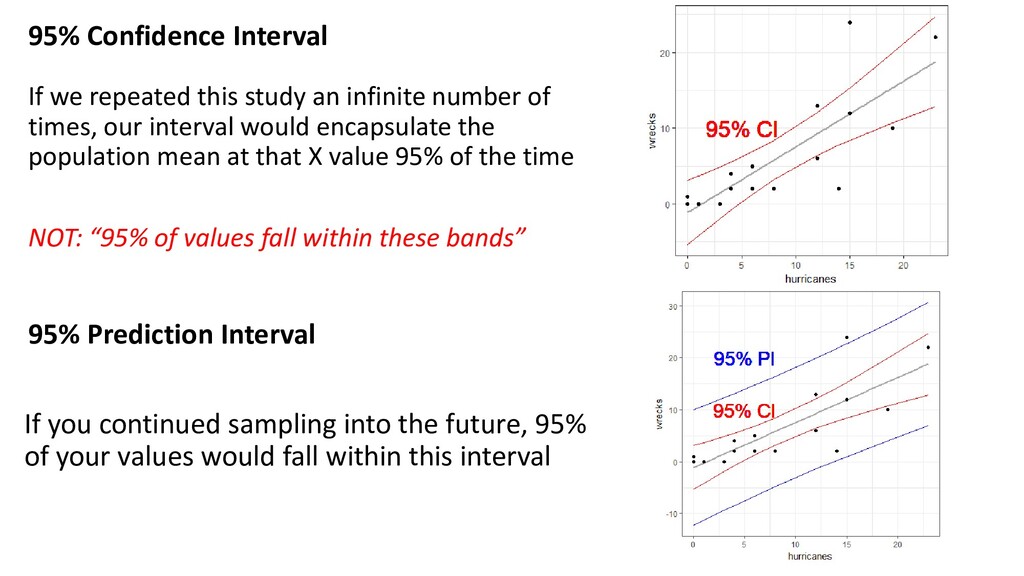
18. 95% Confidence Interval If we repeated this study an infinite number of times, our interval would encapsulate the population mean at that X value 95% of the time NOT: “95% of values fall within these bands” 95% Prediction Interval If you continued sampling into the future, 95% of your values would fall within this interval
19. Here, 95% C.I. of β1 = 0.8657 ± 1.96 * 0.1761 = 0.52 to 1.21 Especially important: 95% CI of Betas of the sample https://en.wikipedia.org/wiki/1.96
20. Interpretation: “For every additional hurricane, there was between 0.52 and 1.21 additional wrecked birds (95% C.I. = 0.87)” β1 Here, 95% C.I. of β1 = 0.8657 ± 1.96 * 0.1761 = 0.52 to 1.21
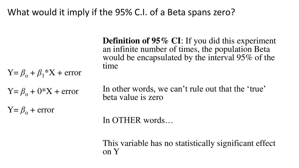
21. What would it imply if the 95% C.I. of a Beta spans zero? Y= βo + β1 *X + error Definition of 95% CI: If you did this experiment an infinite number of times, the population Beta would be encapsulated by the interval 95% of the time In other words, we can’t rule out that the ‘true’ beta value is zero In OTHER words… This variable has no statistically significant effect on Y Y= βo + 0*X + error Y= βo + error
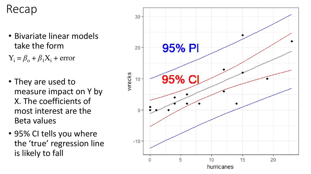
22. Recap • Bivariate linear models take the form Yi = βo + β1 Xi + error • They are used to measure impact on Y by X. The coefficients of most interest are the Beta values • 95% CI tells you where the ‘true’ regression line is likely to fall
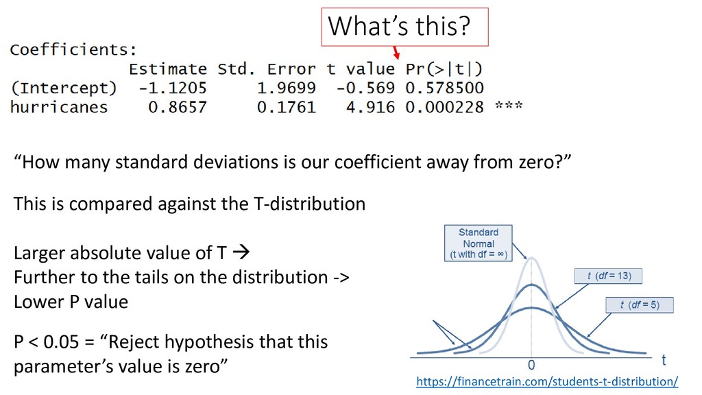
23. What’s this? “How many standard deviations is our coefficient away from zero?” Larger absolute value of T → Further to the tails on the distribution -> Lower P value This is compared against the T-distribution https://financetrain.com/students-t-distribution/ P < 0.05 = “Reject hypothesis that this parameter’s value is zero”
24. Terminology note Parameter: A ‘true’ value from a population – usually unknowable Coefficient: An estimation of the population parameter Parameter estimate: Same as coefficient
25. Assess magnitude of effect on Y Assess significance Assess model fit
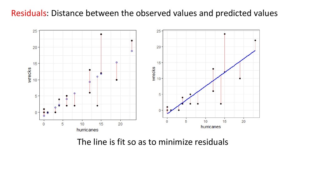
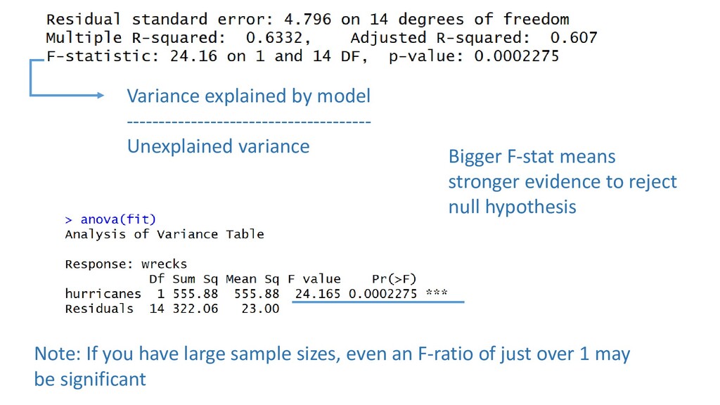
26. Average deviation of observed values from regression line 14 degrees of freedom (df) because... 16 data points 2 coefficients (intercept and slope) So… 16 – 2 = 14 - When R fits a linear regression model, the sum of all residuals adds to zero (intuitively: because there should be as many points “above” line as below, at roughly same overall distance) - Therefore, calculate ‘spread’ of residuals by the following formula:
27. % of variance in Y explainable by X 1 = perfect explanatory power (never happens) 0 = no explanatory power As above, but penalizes model for having additional parameters
28. For simple linear regression only, the square of Pearson’s coefficient is same as R2 • A correlation is the strength of a linear association between two variables r r2 Important: r vs. R2 r = 0: no association r = 1: perfect association
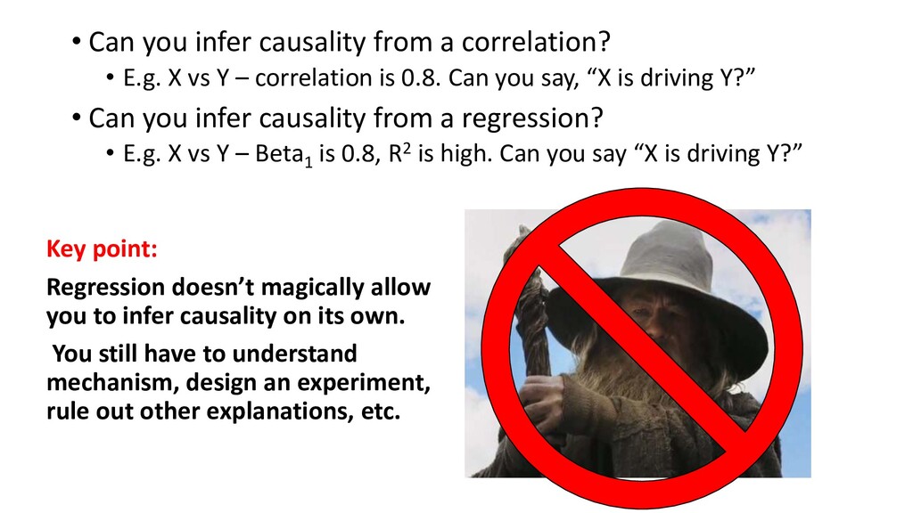
29. • Can you infer causality from a correlation? • E.g. X vs Y – correlation is 0.8. Can you say, “X is driving Y?” • Can you infer causality from a regression? • E.g. X vs Y – Beta1 is 0.8, R2 is high. Can you say “X is driving Y?” Key point: Regression doesn’t magically allow you to infer causality on its own. You still have to understand mechanism, design an experiment, rule out other explanations, etc.
30. Fun with correlations http://guessthecorrelation.com/
31. Variance explained by model -------------------------------------- Unexplained variance Bigger F-stat means stronger evidence to reject null hypothesis Note: If you have large sample sizes, even an F-ratio of just over 1 may be significant
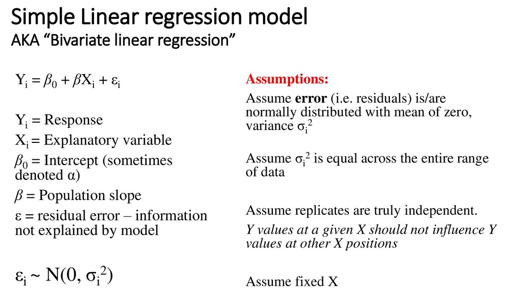
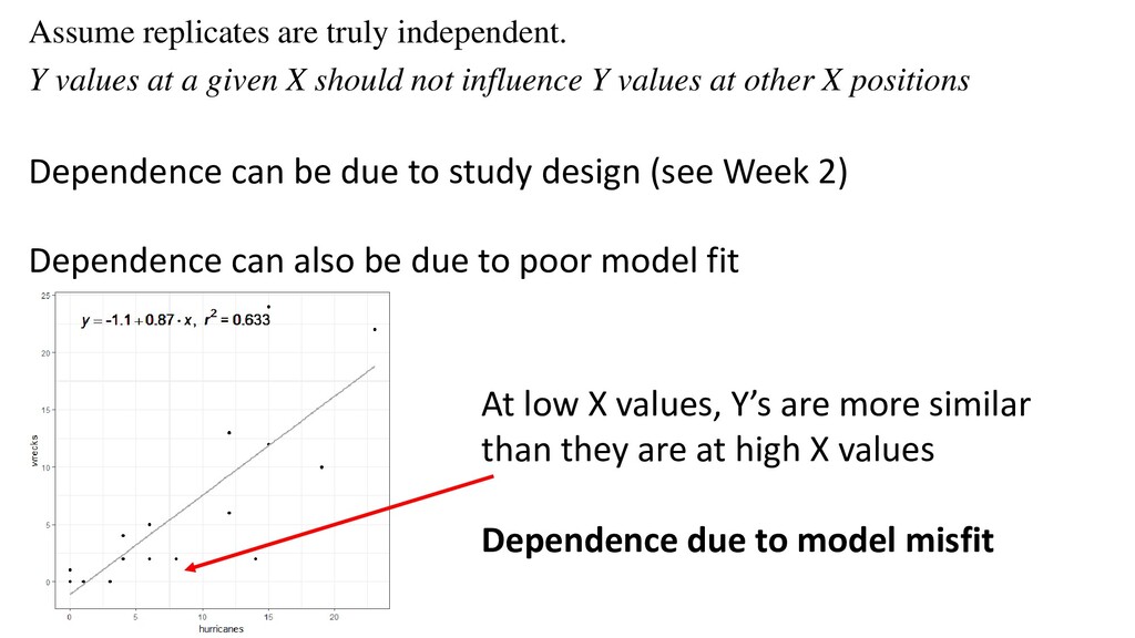
32. Simple Linear regression model Yi = β0 + βXi + εi Yi = Response Xi = Explanatory variable β0 = Intercept (sometimes denoted α) β = Population slope ε = residual error – information not explained by model AKA “Bivariate linear regression” Assumptions: Assume error (i.e. residuals) is/are normally distributed with mean of zero, variance σi 2 Assume σi 2 is equal across the entire range of data Assume replicates are truly independent. Y values at a given X should not influence Y values at other X positions Assume fixed X εi ~ N(0, σi 2)
33. εi ~ N(0, σi 2)  do our data meet this? Yes-ish
34. Assessing Model Fit: Residuals Residuals should be close to normally-distributed
35. Plot residuals vs. fitted values Is σi 2 equal across the entire range of data?
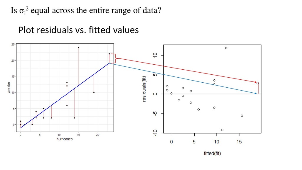
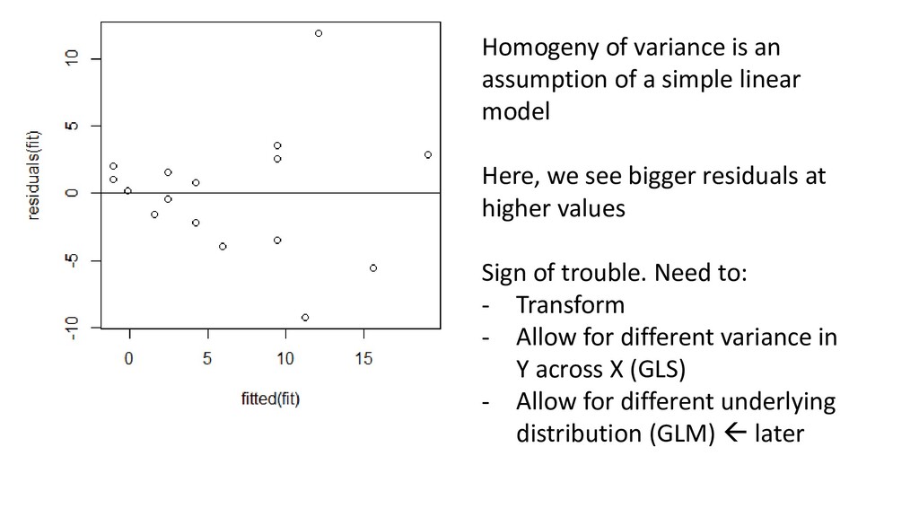
36. Homogeny of variance is an assumption of a simple linear model Here, we see bigger residuals at higher values Sign of trouble. Need to: - Transform - Allow for different variance in Y across X (GLS) - Allow for different underlying distribution (GLM)  later
37. Assume replicates are truly independent. Y values at a given X should not influence Y values at other X positions Dependence can be due to study design (see Week 2) Dependence can also be due to poor model fit At low X values, Y’s are more similar than they are at high X values Dependence due to model misfit
38. Do you see a problem here? Hint: What is our predicted value at low X values? Assessing Model Fit: Watch out for impossible values
39. Q: How did they deal with this in the actual paper? Line does go below zero A: Ignore N.B: Mine looks a bit different because I grabbed values from this plot Huang et al., (2017)
40. Simulate from our model… Draw 50 observations from N(μi , σ2), i.e. our model At fewer than ~12 hurricanes, we are not accurately predicting effect Solution: attend GLM lecture Why does it matter?
41. A few things before we recap… https://www.zoology.ubc.ca/~bio501/lecturepdf/04.Linear%20models.pdf From Dolph Schluter’s UBC Biology 501 notes
42. 1. Simplest version of a linear model is
43. 2. X may be categorical or continuous
44. 1.75 + 9.625 = 11.375
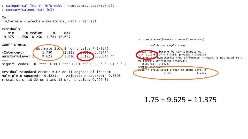
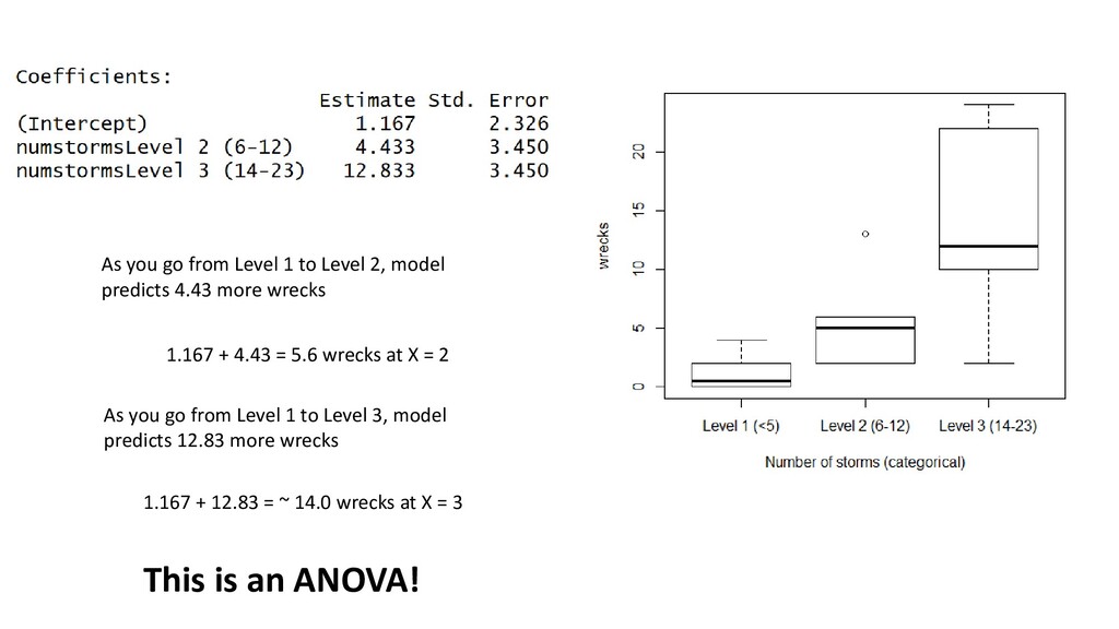
46. As you go from Level 1 to Level 2, model predicts 4.43 more wrecks 1.167 + 4.43 = 5.6 wrecks at X = 2 As you go from Level 1 to Level 3, model predicts 12.83 more wrecks 1.167 + 12.83 = ~ 14.0 wrecks at X = 3 This is an ANOVA!
48. Jonas Kristoffer LindelØv: https://lindeloev.github.io/tests-as-linear/
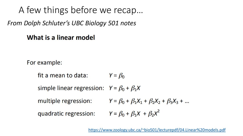
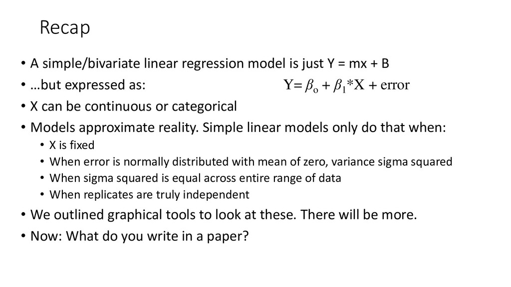
49. Recap • A simple/bivariate linear regression model is just Y = mx + B • …but expressed as: • X can be continuous or categorical • Models approximate reality. Simple linear models only do that when: • X is fixed • When error is normally distributed with mean of zero, variance sigma squared • When sigma squared is equal across entire range of data • When replicates are truly independent • We outlined graphical tools to look at these. There will be more. • Now: What do you write in a paper? Y= βo + β1 *X + error
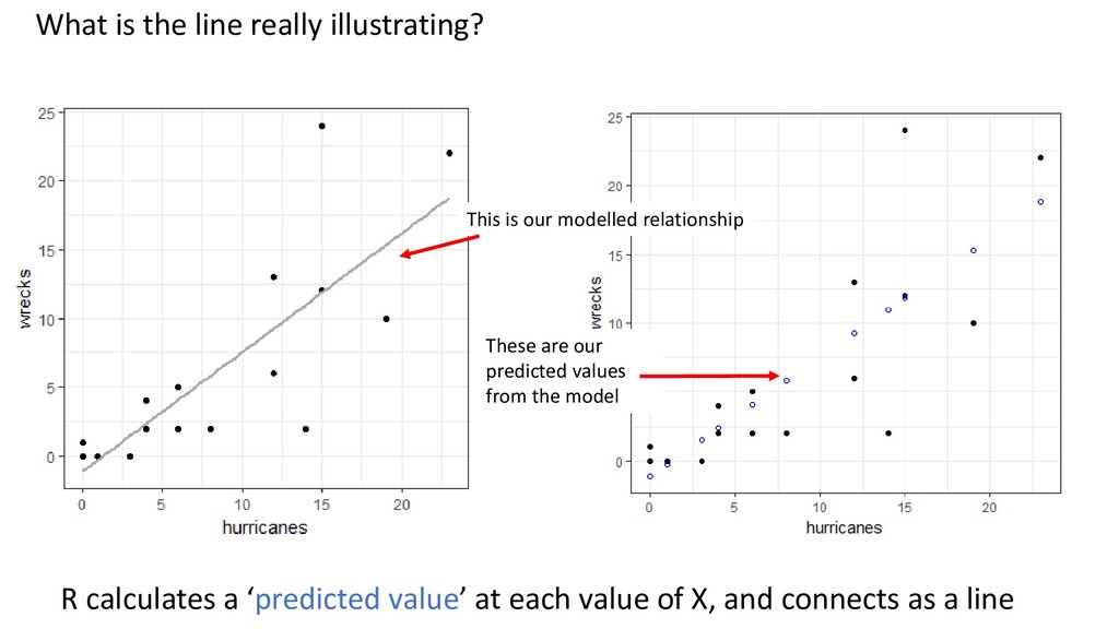
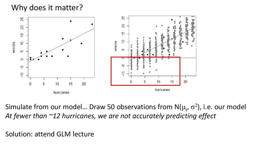
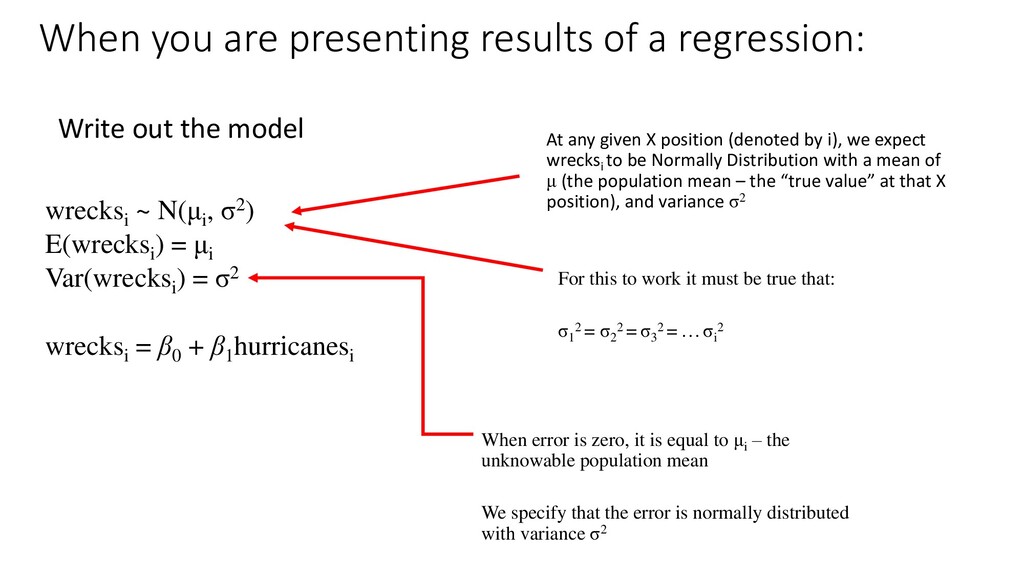
50. When you are presenting results of a regression: At any given X position (denoted by i), we expect wrecksi to be Normally Distribution with a mean of μ (the population mean – the “true value” at that X position), and variance σ2 wrecksi ~ N(μi , σ2) E(wrecksi ) = μi Var(wrecksi ) = σ2 wrecksi = β0 + β1 hurricanesi Write out the model For this to work it must be true that: σ1 2 = σ2 2 = σ3 2 = … σi 2 When error is zero, it is equal to μi – the unknowable population mean We specify that the error is normally distributed with variance σ2
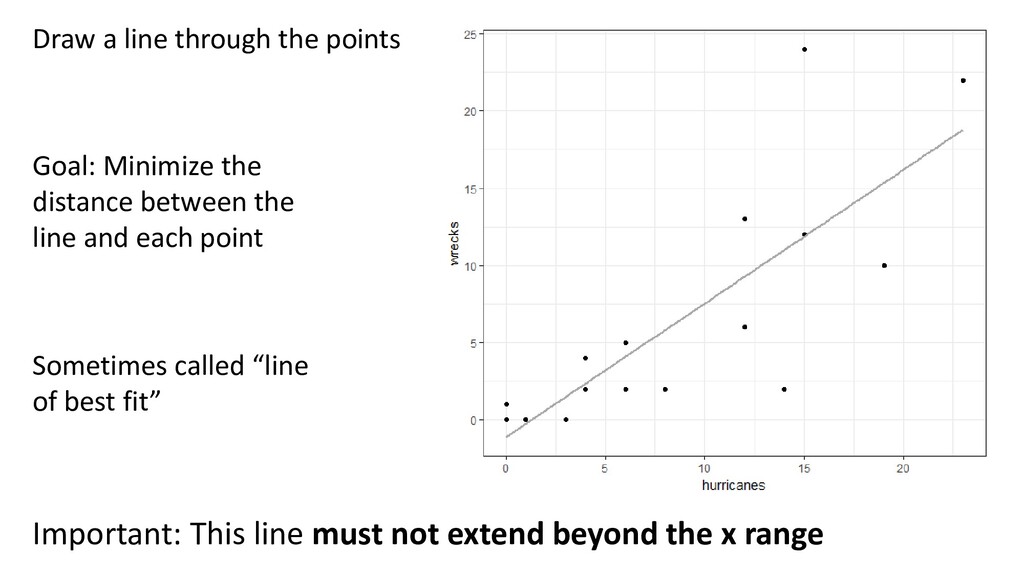
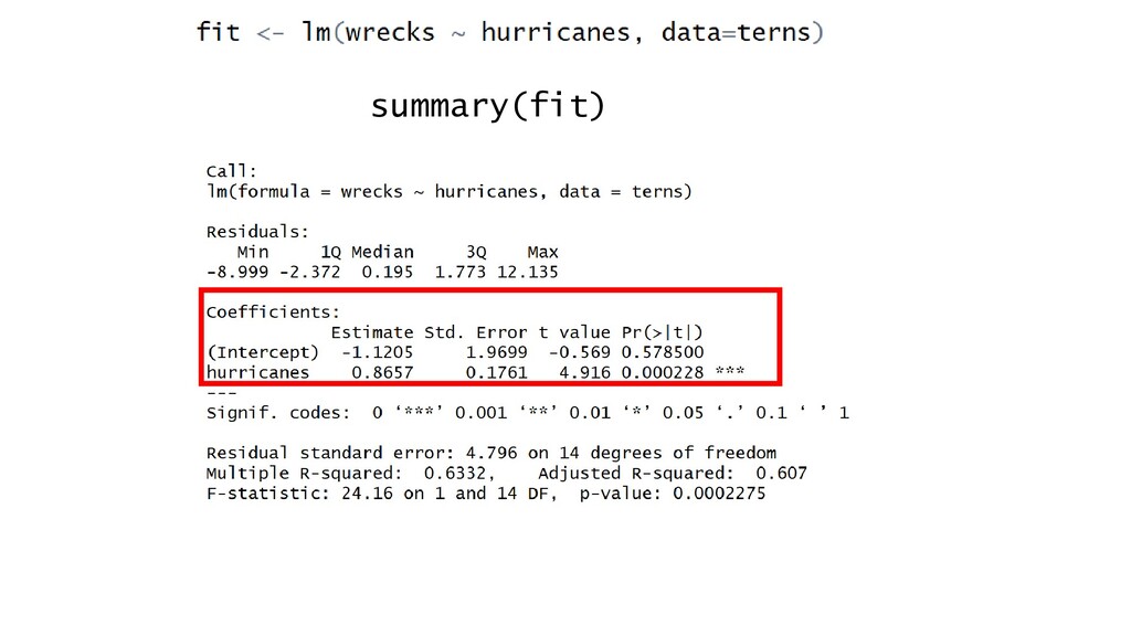
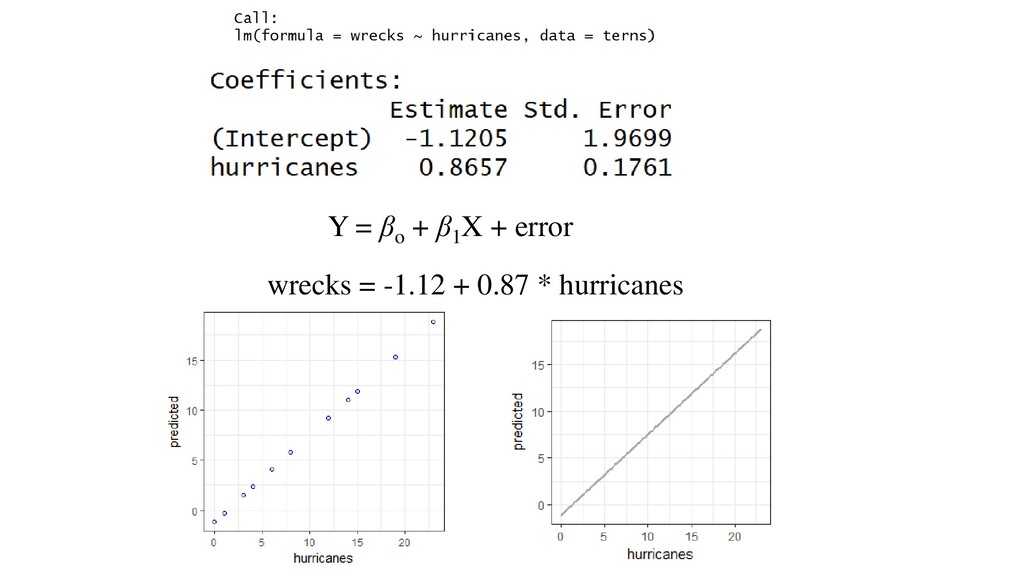
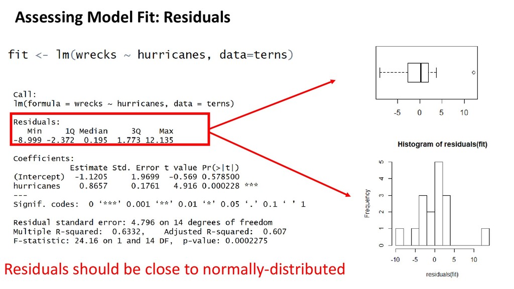
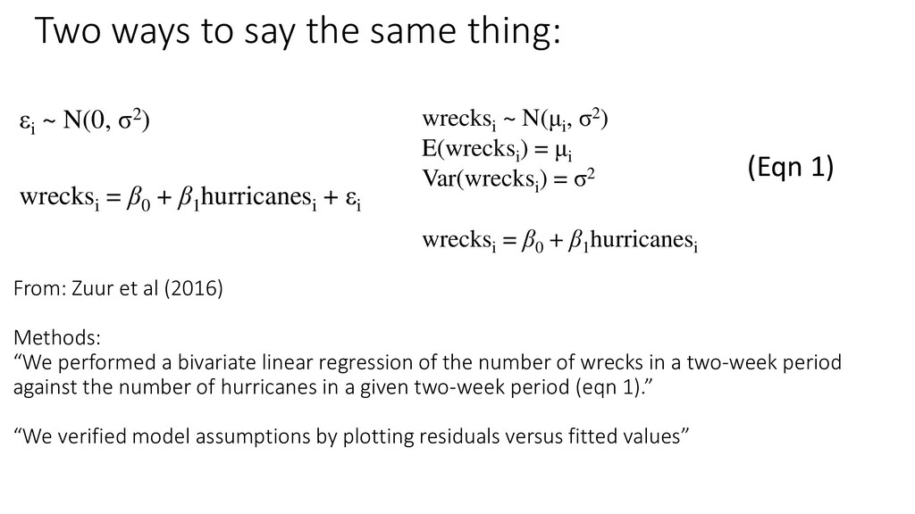
51. εi ~ N(0, σ2) wrecksi = β0 + β1 hurricanesi + εi wrecksi ~ N(μi , σ2) E(wrecksi ) = μi Var(wrecksi ) = σ2 wrecksi = β0 + β1 hurricanesi Two ways to say the same thing: From: Zuur et al (2016) Methods: “We performed a bivariate linear regression of the number of wrecks in a two-week period against the number of hurricanes in a given two-week period (eqn 1).” “We verified model assumptions by plotting residuals versus fitted values” (Eqn 1)
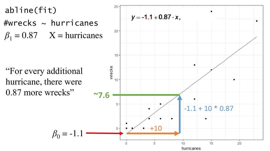
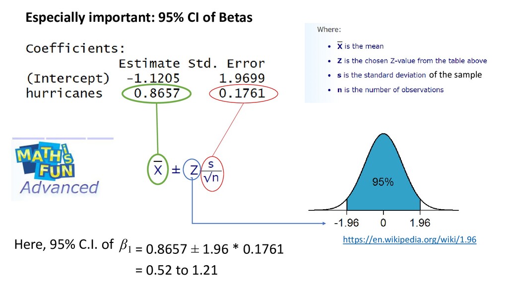
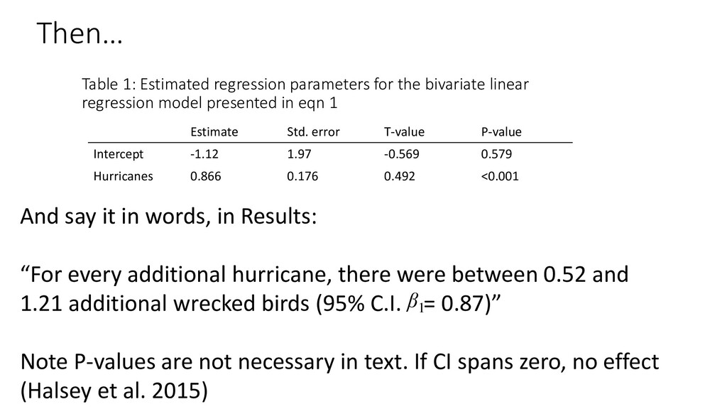
52. Table 1: Estimated regression parameters for the bivariate linear regression model presented in eqn 1 Estimate Std. error T-value P-value Intercept -1.12 1.97 -0.569 0.579 Hurricanes 0.866 0.176 0.492 <0.001 And say it in words, in Results: “For every additional hurricane, there were between 0.52 and 1.21 additional wrecked birds (95% C.I. = 0.87)” Note P-values are not necessary in text. If CI spans zero, no effect (Halsey et al. 2015) Then… β1
53. Next: Visualize the model Figure 1: Fit of the bivariate regression model of wrecks versus hurricanes (eqn 1). Black dots are independent observations, and the blue line indicates predicted model. The grey shading indicates 95% C.I.
54. Why visualize? Analysing Ecological Data Zuur, AF, Ieno, EN, and Smith, GM