FISH 6003: Week 1 Part 2

Part 2 of Week 1

Transcript

1. Week 1: Introduction, and the Philosophy of Statistics Part 2 CatchRate ~ Poisson (μ ij ) E(CatchRate) = μ ij Log(μ ij ) = GearType ij + Temperature ij + FleetDeployment i FleetDeployment i ~ N(0, σ2) Using lme4: m <- glmer(CatchRate ~ GearType + Temperature + (1 | FleetDeployment), family = poisson) FISH 6003 FISH 6000: Science Communication for Fisheries Brett Favaro 2017 This work is licensed under a Creative Commons Attribution 4.0 International License
2. This week: • Introduction to the course • Introduction to assignments • What are statistics? • Working with an R project – and boxplots • Defining terms • Statistical thinking
3. Statistics A discipline of mathematics focused on describing and deriving information from data. It turns this: Into this:
4. Statistics are used in science to help us answer questions: • Did my experimental treatment have an impact? • Did my new fishing gear cause a REAL increase in catch rates? Or was it due to chance alone? • How much of an impact did my treatment have? (MAGNITUDE and DIRECTION of an effect) • Was my fishing gear 5% responsible for increased catch rates? 25%? Something else? • How much did my treatment matter, versus other potential factors? • Was it my new fishing gear that improved catch rates, or something else? • What is the weight of evidence on a given topic? • MY study found the gear increased catch by 25%. What did other studies find? Can we expect ANYONE to see a 25% increase in catch if they use my gear? Statistics allow you to derive defensible conclusions from your data
5. https://cesess.wordpress.com/2015/08/03/on-the-appropriate-use-of-statistics-in-ecology- an-interview-with-ben-bolker/ H: Why do we need statistics in ecology? B: Because the world is noisy. Because the world is noisy and because scientists are conservative. If I do my experiment and all 20 control animals die and all 20 treatment animals survive I don’t need statistics to tell me the treatment had an effect. But if 14 of the control animals die and 10 of the treatment animals die, well, I don’t know. Did the treatment have an effect? At some point you are going to have to draw a line, and you are also going to draw a line that the community will accept. You can’t just say “Well, it looks to me like my treatment was successful”. Statistics is the community standard.
6. Statistical Refresher This, and next few slides: Halsey et al. (2015): The fickle P value generates irreproducible results Descriptive statistics Descriptors of the basic features of data - Mean, median, mode, range, standard deviation
7. In some papers, descriptive statistics are all you need
8. Probability distribution A mathematical function where the area under the curve = 1 Normal (Gaussian) distribution, defined by: Mean μ Standard deviation σ https://upload.wikimedia.org/wikipedia/commons/thumb/a/a 9/Empirical_Rule.PNG/450px-Empirical_Rule.PNG
9. Probability distribution Gaussian: Mean μ Standard deviation σ https://upload.wikimedia.org/wikipedia/commons/thumb/a/a 9/Empirical_Rule.PNG/450px-Empirical_Rule.PNG In statistics
10. Go to: http://homepage.divms.uiowa.edu/~mbognar/applets/normal.html - Imagine an infinite number of people taking an aptitude test. The mean value of the test is 10. SD is 1. - If someone scored exactly 10, they would be in the 50th percentile and their score would be greater than 50% percent of the population.
11. Go to: http://homepage.divms.uiowa.edu/~mbognar/applets/normal.html - Randomly draw one person to take the test - What is the probability that they will score exactly 10? - What is the probability they will score 10 or less? - What is the probability they will score 9? - 9 or less? - 9 or more?
12. Imagine we randomly give people this test. What will their scores be?
13. Imagine we randomly give people this test. What will their scores be?
14. Imagine we randomly give people this test. What will their scores be?
15. These are called “sampling distributions,” AKA frequency distribution. The more we sample, the closer we get to the population mean and standard deviation. Imagine we randomly give people this test. What will their scores be?
16. Probability distribution Sampling distribution/Frequency distributions Describes a population Describes a sample
17. Randomly measure 100 people’s scores Replot as probabilities
18. Population: N(μ = 10, σ = 1) N(10, 1)  a normal curve with μ = 10, σ = 1
19. Population: N(μ = 10, σ = 1) N(10, 1)  a normal curve with μ = 10, σ = 1 Sample: n = 100 Sample mean: x̄ = 9.87
20. Population: N(μ = 10, σ = 1) N(10, 1)  a normal curve with μ = 10, σ = 1 Sample: n = 100 Sample mean: x̄ = 9.87 Standard Error of Sample: The standard deviation of the sampling distribution
21. Standard error of sample can also be called: Standard deviation of sample Standard deviation of sampling distribution Standard error NOT TO BE CONFUSED WITH: Standard error of the mean (coming soon)
22. Probability distribution Sampling distribution/Frequency distributions Population Sample Spread = standard deviation Spread = Standard error
23. Calculating standard error of sample “Sample 100 random observations from a normally distributed population with μ = 10, σ = 1” Recall: sd(y) # Is this calculating σ or s?
24. Answer: 1.y is a SAMPLE. So we can’t be measuring σ 2. From help(sd) sd(y) # Is this calculating σ or s? Lesson: Know what R is doing. Use precise terms
25. Hasley et al (2015) Most other resources Sample variance This is known as “Bessel’s Correction”
26. Sample: n = 100 Sample mean: x̄ = 9.87 Standard Error of Sample: 1.072
27. Sample: n = 100 Sample mean: x̄ = 9.87 Standard Error of Sample: 1.072
28. Sample: n = 100 Sample mean: x̄ = 9.87 Standard Error of Sample: 1.072 ± 1 S.E. Encompasses 68% of data (if normally distributed)
29. Sample: n = 100 Sample mean: x̄ = 9.87 Standard Error of Sample: 1.072 ± 1 S.E. Encompasses 68% of data (if normally distributed) ± 2 S.E. Encompasses ~95% of data (if normally distributed)
30. Sample: n = 100 Sample mean: x̄ = 9.87 Standard Error of Sample: 1.072 Standard Error of Mean (not the same thing!)
31. Sample: n = 100 Sample mean: x̄ = 9.87 Standard Error of Sample: 1.072 Standard Error of Mean: 1.072 / sqrt(100) = 0.107 Note: What happens to SEM if n goes up?
32. Sample: n = 100 Sample mean: x̄ = 9.87 Standard Error of Sample: 1.072 Standard Error of Mean: 0.107 ± 1 S.E.M
33. Sample: n = 100 Sample mean: x̄ = 9.87 Standard Error of Sample: 1.072 Standard Error of Mean: 0.107 ± 1 S.E.M ± 2 S.E.M
34. Go to: http://www.zoology.ubc.ca/~whitlock/Kingfisher/SamplingNor mal.htm
35. Sample: n = 100 Sample mean: x̄ = 9.87 Standard Error of Sample: 1.072 Standard Error of Mean: 0.107 95% Confidence Interval: The range of values around an estimate that, if sampled 20 times, would contain the population mean 19 times. What is mean ± 1.96 * S.E.M. ?
36. Here, I sampled from a normally distributed population with mean = 10, sd = 1. This is mean and 95% CI for 20 samples of 100 19 times out of 20, the CI encompassed the ‘true mean’ (i.e. the population mean)
37. If you report properly, standard error and SEM can be calculated from each other • If you report s and n, you can calculate SEM • If you report SEM and n, you can calculate s • If you don’t report n…
39. Descriptive statistics Descriptors of the basic features of data - Mean, median, mode, range, standard deviation Mean: Vulnerable to non-normality Example: Mean household income in the United States in 2014 = $74,641 But tail is long: Median: $53,700
40. McCune et al. (2017) – Assessing public commitment to endangered species protection: A Canadian case study. FACETS Journal: facetsjournal.com/article/facets-2016-0054/ These are “Likert” data. Why not just report a mean? Hint: What is the average of “Strongly agree” and “strongly disagree?”
41. Recap • Mean, median, mode • Population mean, standard deviation • Sample mean, standard error, standard error of the mean • Realistically, when most people say S.E., they really mean S.E.M. • Know when to use each: • SE for describing dispersion of data • SEM for computing confidence intervals from model output
42. Median (2nd quartile) 25%, 1st quartile 75%, 3rd quartile Outlier Boxplots Imagine ten Atlantic salmon. We measure the total length of each individual fish in cm. Visualize with a boxplot (flipped on its side) Salmon by parkjisun from the Noun Project Total length
43. Median (Q2) 50th percentile (everything below this = 50% of data) Q1 – First Quartile 25th percentile (i.e. everything below this = 25% of data) Q3 – Third quartile 75th percentile (everything below this = 75% of data) Quartiles: Three points that divide data into four equal groups i.e. ¼ of data in each quartile
44. Quartiles: Three points that divide data into four equal groups i.e. ¼ of data in each quartile Ten values: *If there is an even number of items, median = mean of middle two numbers Values 5 and 6 are central* 5th value = 45 6th value = 46 (45 + 46) /2 = 45.5 Question: What is the median?
45. Quartiles: Three points that divide data into four equal groups i.e. ¼ of data in each quartile Ten values: Question: What is Q1 and Q3? How is R doing this? help(geom_boxplot)
46. Details The two ‘hinges’ are versions of the first and third quartile, i.e., close to quantile(x, c(1,3)/4). The hinges equal the quartiles for odd n (where n <- length(x)) and differ for even n. Whereas the quartiles only equal observations for n %% 4 == 1 (n = 1 mod 4), the hinges do so additionally for n %% 4 == 2 (n = 2 mod 4), and are in the middle of two observations otherwise. The notches (if requested) extend to +/-1.58 IQR/sqrt(n). This seems to be based on the same calculations as the formula with 1.57 in Chambers et al (1983, p. 62), given in McGill et al (1978, p. 16). They are based on asymptotic normality of the median and roughly equal sample sizes for the two medians being compared, and are said to be rather insensitive to the underlying distributions of the samples. The idea appears to be to give roughly a 95% confidence interval for the difference in two medians. help(geom_boxplot) help(boxplot.stats) Summary statistics The lower and upper hinges correspond to the first and third quartiles (the 25th and 75th percentiles). This differs slightly from the method used by the boxplot function [i.e. the R base boxplot function], and may be apparent with small samples. See boxplot.stats for for more information on how hinge positions are calculated for boxplot. ggplot2 and base plot may produce slightly different boxplots from the same data!
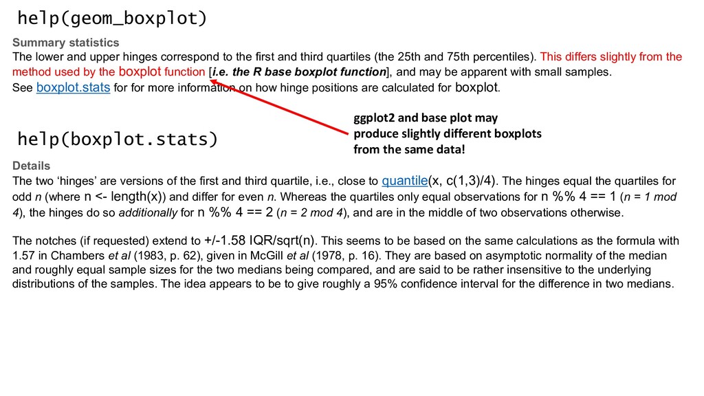
47. Types quantile returns estimates of underlying distribution quantiles based on one or two order statistics from the supplied elements in x at probabilities in probs. One of the nine quantile algorithms discussed in Hyndman and Fan (1996), selected by type, is employed. All sample quantiles are defined as weighted averages of consecutive order statistics. Sample quantiles of type i are defined by: Q[i](p) = (1 - γ) x[j] + γ x[j+1], where 1 ≤ i ≤ 9, (j-m)/n ≤ p < (j-m+1)/n, x[j] is the jth order statistic, n is the sample size, the value of γ is a function of j = floor(np + m) and g = np + m - j, and m is a constant determined by the sample quantile type. Discontinuous sample quantile types 1, 2, and 3 For types 1, 2 and 3, Q[i](p) is a discontinuous function of p, with m = 0 when i = 1 and i = 2, and m = -1/2when i = 3. Type 1 Inverse of empirical distribution function. γ = 0 if g = 0, and 1 otherwise. Type 2 Similar to type 1 but with averaging at discontinuities. γ = 0.5 if g = 0, and 1 otherwise. Type 3 SAS definition: nearest even order statistic. γ = 0 if g = 0 and j is even, and 1 otherwise. Continuous sample quantile types 4 through 9 For types 4 through 9, Q[i](p) is a continuous function of p, with gamma = g and m given below. The sample quantiles can be obtained equivalently by linear interpolation between the points (p[k],x[k]) where x[k] is thekth order statistic. Specific expressions for p[k] are given below. Type 4 m = 0. p[k] = k / n. That is, linear interpolation of the empirical cdf. Type 5 m = 1/2. p[k] = (k - 0.5) / n. That is a piecewise linear function where the knots are the values midway through the steps of the empirical cdf. This is popular amongst hydrologists. Type 6 m = p. p[k] = k / (n + 1). Thus p[k] = E[F(x[k])]. This is used by Minitab and by SPSS. Type 7 m = 1-p. p[k] = (k - 1) / (n - 1). In this case, p[k] = mode[F(x[k])]. This is used by S. Type 8 m = (p+1)/3. p[k] = (k - 1/3) / (n + 1/3). Then p[k] =~ median[F(x[k])]. The resulting quantile estimates are approximately median-unbiased regardless of the distribution of x. Type 9 m = p/4 + 3/8. p[k] = (k - 3/8) / (n + 1/4). The resulting quantile estimates are approximately unbiased for the expected order statistics if x is normally distributed. Further details are provided in Hyndman and Fan (1996) who recommended type 8. The default method is type 7, as used by S and by R < 2.0.0. help(quantile)
48. 3. Stats software (and packages) calculate things slightly differently. This is why it’s critical to state what software and packages you used to conduct analysis, produce plots, etc. At least R is transparent about this… Lessons: 1. A lot of computations happen in the background. Nine possible types of Q1 and Q3!! 2. Use help() to figure out what’s going on
49. Quartiles: Three points that divide data into four equal groups i.e. ¼ of data in each quartile Ten values: Question: What are the whiskers? InterQuartile Range (IQR) = Q3 – Q1 = 46.75 – 41.5 = 5.25 Upper whisker = Q3 + 1.5 * IQR = 46.75 + 1.5 * (5.25) = 54.6 But there’s no 54.6! Whisker extends as high as, but no higher, than 54.6 Highest is 50 – so upper end of whisker is 50
50. Quartiles: Three points that divide data into four equal groups i.e. ¼ of data in each quartile Ten values: Question: What are the whiskers? Lower whisker = Q1 - 1.5 * IQR = 41.5 - 1.5 * (5.25) = 33.6 We don’t have a 33.6. Closest is 38 Lower whisker extends as low as, but no lower, than 33.6 Therefore, lower whisker is 38 31, which is less than 33.6, becomes an outlier!
51. Take-home message: • A boxplot is a powerful way to visualize data. On a quick glance, you get spread and central value of a categorical variable • But, all data visualizations, all models, etc. make assumptions, and engage in calculations. Be mindful of how this affects interpretation • Key: All these factors are customizable (e.g. you could calculate Q’s differently). If you change defaults, ALWAYS disclose what you did, and why.
52. Quartiles, median, etc. are calculated by position in a series of numbers. How many pieces of data are plotted here? SE, SEM, are calculated based on the magnitude of all the values in the sample. Recall n = 100. How many pieces of data are plotted here?
53. Recap • Boxplots are a common data visualization tool: but all dataviz tools have underlying assumptions and computations • R has a ton of features. Know what you’re doing when you use them! • Always report what software, packages, etc. you used to make plots, do analysis, and so on • If you change default settings, DISCLOSE in your paper
54. P-values • Probability: The proportion of times an event would occur if it was hypothetically repeated an infinite number of times, all else being equal Inferential Statistics: Any statistical technique where you use a sample to infer something about a general population “The treatment had an effect in our study, therefore it is likely to produce a similar effect if used outside this study”  whatever technique was used to back this up is an inferential statistic
55. • In your undergraduate stats course, you learned about frequentist statistics • All these techniques share a common logic: • Everything is based on disproving a “Null Hypothesis” – that there is no relationship between the variables being examined. • Key parameter of interest: • Probability of getting your results, assuming the null hypothesis was true • Example in words: What is the probability that I would see this difference between treatment group A and B, if in reality there was no difference? • If the probability is low (less than 0.05), consider it to be “statistically significant” • P <= 0.05 = “statistically significant.” Reject Ho . Rejoice. • P > 0.05 = “Not statistically significant.” Do not reject Ho . Despair. • P-Values communicate the strength of evidence against Ho . They do not communicate the magnitude of an effect.
56. Quiz: In Study A, I had a P-value of 0.04. In Study B, I had a P-value of 0.0001. Which study has stronger statistical evidence to reject Ho ? In which study did our treatment have a bigger effect?
57. P-value • The P-value is the probability of observing the divergence from Ho that you observed in your data, assuming Ho is true • The P-value is often treated like a binary switch. Something IS or ISN’T ‘significant’ and that’s the end of it • That’s not enough Looking ahead: - See course website for some additional wisdom re: P-values
58. Your turn! Please download FISH6003_Week1_Intro.zip from the course website Unzip it somewhere on your computer
59. Open this in R Studio *Switch to R Studio, walk through project*