Can We Solve It? If So, How Fast?

General talk about adaptive algorithms

Transcript

1. Can We Solve It? If So, How Fast? Fred J. Hickernell Department of Applied Mathematics Center for Interdisciplinary Scientific Computation Illinois Institute of Technology hickernell@iit.edu mypages.iit.edu/~hickernell Thanks to my friends and collaborators, including the GAIL team and also NSF-DMS-1522687 and NSF-DMS-1638521 (SAMSI) Computational Mathematics and Statistics Seminar, September 13, 2018
2. Introduction Solvability Optimality Adaptive Algorithms Open Problems References What Does It Mean to Solve a Mathematics or Statistics Problem? Problem Solution x2 + 2x − 3 = 0 x = −3, 1 numbers 2/13
3. Introduction Solvability Optimality Adaptive Algorithms Open Problems References What Does It Mean to Solve a Mathematics or Statistics Problem? Problem Solution x2 + 2x − 3 = 0 x = −3, 1 numbers d dx sin(x) cos(x) elementary function 2/13
4. Introduction Solvability Optimality Adaptive Algorithms Open Problems References What Does It Mean to Solve a Mathematics or Statistics Problem? Problem Solution x2 + 2x − 3 = 0 x = −3, 1 numbers d dx sin(x) cos(x) elementary function 1 √ 2π 1 −∞ e−x2/2 dx Φ(1) special function Φ is the standard Gaussian cumulative distribution function 2/13
5. Introduction Solvability Optimality Adaptive Algorithms Open Problems References What Does It Mean to Solve a Mathematics or Statistics Problem? Problem Solution x2 + 2x − 3 = 0 x = −3, 1 numbers d dx sin(x) cos(x) elementary function 1 √ 2π 1 −∞ e−x2/2 dx Φ(1) special function Φ is the standard Gaussian cumulative distribution function 1 0 f(x) dx Need a numerical solution, i.e., A(f, ε) f known via an algorithm depending on integrand values f(x1), f(x2), . . . i.e., can get f(x) ∀x ∈ [0, 1] such that 1 0 f(x) dx − A(f, ε) ε 2/13
6. Introduction Solvability Optimality Adaptive Algorithms Open Problems References What About the Trapezoidal Rule? 1 0 f(x) dx ≈ Tn(f) = 1 n f(0) 2 + f 1 n + · · · + f n − 1 n + f(1) 2 T1(f) = 0.5034 3/13
7. Introduction Solvability Optimality Adaptive Algorithms Open Problems References What About the Trapezoidal Rule? 1 0 f(x) dx ≈ Tn(f) = 1 n f(0) 2 + f 1 n + · · · + f n − 1 n + f(1) 2 T2(f) = 0.3949 3/13
8. Introduction Solvability Optimality Adaptive Algorithms Open Problems References What About the Trapezoidal Rule? 1 0 f(x) dx ≈ Tn(f) = 1 n f(0) 2 + f 1 n + · · · + f n − 1 n + f(1) 2 T4(f) = 0.3954 3/13
9. Introduction Solvability Optimality Adaptive Algorithms Open Problems References What About the Trapezoidal Rule? 1 0 f(x) dx ≈ Tn(f) = 1 n f(0) 2 + f 1 n + · · · + f n − 1 n + f(1) 2 T50(f) = 0.3957 3/13
10. Introduction Solvability Optimality Adaptive Algorithms Open Problems References What About the Trapezoidal Rule? 1 0 f(x) dx ≈ Tn(f) = 1 n f(0) 2 + f 1 n + · · · + f n − 1 n + f(1) 2 Theory says 1 0 f(x) dx − Tn(f) curvature 1 0 f (x) dx 8n2 = f 1 8n2 ? ε T50(f) = 0.3957 3/13
11. Introduction Solvability Optimality Adaptive Algorithms Open Problems References What About the Trapezoidal Rule? 1 0 f(x) dx ≈ Tn(f) = 1 n f(0) 2 + f 1 n + · · · + f n − 1 n + f(1) 2 Theory says 1 0 f(x) dx − Tn(f) curvature 1 0 f (x) dx 8n2 = f 1 8n2 ? ε Let F = {f : f 1 ρ} , and let A(f, ε) = Tn(f) where n = ρ 8ε Then 1 0 f(x) dx − A(f, ε) ε ∀f ∈ F, ε > 0 T50(f) = 0.3957 3/13
12. Introduction Solvability Optimality Adaptive Algorithms Open Problems References What About the Trapezoidal Rule? 1 0 f(x) dx ≈ Tn(f) = 1 n f(0) 2 + f 1 n + · · · + f n − 1 n + f(1) 2 Let A(f, ε) = Tn(f) where n = ρ 8ε Then 1 0 f(x) dx − A(f, ε) ε ∀f ∈ F = {f : f 1 ρ}, ε > 0 T50(f) = 0.3957 We say that integration is solvable for integrands in F 3/13
13. Introduction Solvability Optimality Adaptive Algorithms Open Problems References Solvability A problem is called solvable for a set of inputs F if there exists a numerical algorithm that provides a solution with error no greater than ε. Specifically, integration is solvable for F if there exists an A for which 1 0 f(x) dx − A(f, ε) ε ∀f ∈ F, ε > 0 Kunsch, R. J., Novak, E. & Rudolf, D. Solvable Integration Problems and Optimal Sample Size Selection. submitted for publication. 2018+. 4/13
14. Introduction Solvability Optimality Adaptive Algorithms Open Problems References Solvability A problem is called solvable for a set of inputs F if there exists a numerical algorithm that provides a solution with error no greater than ε. Specifically, integration is solvable for F if there exists an A for which 1 0 f(x) dx − A(f, ε) ε ∀f ∈ F, ε > 0 We demonstrated that integration is solvable for F = {f : f 1 ρ} Kunsch, R. J., Novak, E. & Rudolf, D. Solvable Integration Problems and Optimal Sample Size Selection. submitted for publication. 2018+. 4/13
15. Introduction Solvability Optimality Adaptive Algorithms Open Problems References Solvability A problem is called solvable for a set of inputs F if there exists a numerical algorithm that provides a solution with error no greater than ε. Specifically, integration is solvable for F if there exists an A for which 1 0 f(x) dx − A(f, ε) ε ∀f ∈ F, ε > 0 We demonstrated that integration is solvable for F = {f : f 1 ρ} Is integration solvable for F = {f : f 1 < ∞} since 1 0 f(x) dx − Tn(f) f 1 8n2 ? Kunsch, R. J., Novak, E. & Rudolf, D. Solvable Integration Problems and Optimal Sample Size Selection. submitted for publication. 2018+. 4/13
16. Introduction Solvability Optimality Adaptive Algorithms Open Problems References Integration Is Not Solvable for F = {f : f 1 < ∞} Suppose that there exists A such that 1 0 f(x) dx − A(f, ε) ε ∀f ∈ F = {f : f 1 < ∞}, ε > 0 5/13
17. Introduction Solvability Optimality Adaptive Algorithms Open Problems References Integration Is Not Solvable for F = {f : f 1 < ∞} Suppose that there exists A such that 1 0 f(x) dx − A(f, ε) ε ∀f ∈ F = {f : f 1 < ∞}, ε > 0 Observe where A(0, ε) gets function values 5/13
18. Introduction Solvability Optimality Adaptive Algorithms Open Problems References Integration Is Not Solvable for F = {f : f 1 < ∞} Suppose that there exists A such that 1 0 f(x) dx − A(f, ε) ε ∀f ∈ F = {f : f 1 < ∞}, ε > 0 Observe where A(0, ε) gets function values Construct fbump ∈ F, as tall as you like; note that A(0, ε) = A(fbump , ε) 5/13
19. Introduction Solvability Optimality Adaptive Algorithms Open Problems References Integration Is Not Solvable for F = {f : f 1 < ∞} Suppose that there exists A such that 1 0 f(x) dx − A(f, ε) ε ∀f ∈ F = {f : f 1 < ∞}, ε > 0 Observe where A(0, ε) gets function values Construct fbump ∈ F, as tall as you like; note that A(0, ε) = A(fbump , ε) Since 1 0 0 dx and 1 0 fbump (x) dx are so different, A cannot be successful 5/13
20. Introduction Solvability Optimality Adaptive Algorithms Open Problems References Integration Is Not Solvable for F = {f : f 1 < ∞} Suppose that there exists A such that 1 0 f(x) dx − A(f, ε) ε ∀f ∈ F = {f : f 1 < ∞}, ε > 0 Observe where A(0, ε) gets function values Construct fbump ∈ F, as tall as you like; note that A(0, ε) = A(fbump , ε) Since 1 0 0 dx and 1 0 fbump (x) dx are so different, A cannot be successful Why doesn’t this argument hold for F = {f : f 1 ρ} ? 5/13
21. Introduction Solvability Optimality Adaptive Algorithms Open Problems References Integration Is Not Solvable for F = {f : f 1 < ∞} Suppose that there exists A such that 1 0 f(x) dx − A(f, ε) ε ∀f ∈ F = {f : f 1 < ∞}, ε > 0 Observe where A(0, ε) gets function values Construct fbump ∈ F, as tall as you like; note that A(0, ε) = A(fbump , ε) Since 1 0 0 dx and 1 0 fbump (x) dx are so different, A cannot be successful Why doesn’t this argument hold for F = {f : f 1 ρ} ? Because fbump / ∈ 5/13
22. Introduction Solvability Optimality Adaptive Algorithms Open Problems References Is Trapezoidal Rule the Best Algorithm? Let cost(A, f, ε) denote the number of function values, n required for A(f, ε) and cost(A, F, ε) = sup f∈F cost(A, f, ε) For our trapezoidal rule algorithm, A cost(A, F, ε) = cost(A, f, ε) = ρ 8ε = O ρ ε ∀f ∈ F = {f : f 1 ρ} This is the (up to a constant) the smallest possible cost 6/13
23. Introduction Solvability Optimality Adaptive Algorithms Open Problems References Is Trapezoidal Rule the Best Algorithm? Let cost(A, f, ε) denote the number of function values, n required for A(f, ε) and cost(A, F, ε) = sup f∈F cost(A, f, ε) For our trapezoidal rule algorithm, A cost(A, F, ε) = cost(A, f, ε) = ρ 8ε = O ρ ε ∀f ∈ F = {f : f 1 ρ} This is the (up to a constant) the smallest possible cost for integrands in F = {f : f 1 ρ} , no worse than Simpson’s rule, Gauss rules, etc. 6/13
24. Introduction Solvability Optimality Adaptive Algorithms Open Problems References Why the Trapezoidal Rule Is Optimal for F = {f : f 1 < ρ} Let A be any algorithm satisfying 1 0 f(x) dx − A(f, ε) ε ∀f ∈ F = {f : f 1 < ρ}, ε > 0 7/13
25. Introduction Solvability Optimality Adaptive Algorithms Open Problems References Why the Trapezoidal Rule Is Optimal for F = {f : f 1 < ρ} Let A be any algorithm satisfying 1 0 f(x) dx − A(f, ε) ε ∀f ∈ F = {f : f 1 < ρ}, ε > 0 Observe where A(0, ε) gets function values 7/13
26. Introduction Solvability Optimality Adaptive Algorithms Open Problems References Why the Trapezoidal Rule Is Optimal for F = {f : f 1 < ρ} Let A be any algorithm satisfying 1 0 f(x) dx − A(f, ε) ε ∀f ∈ F = {f : f 1 < ρ}, ε > 0 Observe where A(0, ε) gets function values Construct fbump ∈ F; note that A(0, ε) = A(fbump , ε) = A(−fbump , ε) 7/13
27. Introduction Solvability Optimality Adaptive Algorithms Open Problems References Why the Trapezoidal Rule Is Optimal for F = {f : f 1 < ρ} Let A be any algorithm satisfying 1 0 f(x) dx − A(f, ε) ε ∀f ∈ F = {f : f 1 < ρ}, ε > 0 Observe where A(0, ε) gets function values Construct fbump ∈ F; note that A(0, ε) = A(fbump , ε) = A(−fbump , ε) For A to succeed for ±fbump , which have different integrals, one must have cost(A, F, ε) = O ρ ε the same as the trapezoidal rule algorithm. 7/13
28. Introduction Solvability Optimality Adaptive Algorithms Open Problems References Why the Trapezoidal Rule Is Optimal for F = {f : f 1 < ρ} Let A be any algorithm satisfying 1 0 f(x) dx − A(f, ε) ε ∀f ∈ F = {f : f 1 < ρ}, ε > 0 Observe where A(0, ε) gets function values Construct fbump ∈ F; note that A(0, ε) = A(fbump , ε) = A(−fbump , ε) For A to succeed for ±fbump , which have different integrals, one must have cost(A, F, ε) = O ρ ε the same as the trapezoidal rule algorithm. Why do your instructors tell you that other algorithms are better than the trapezoidal rule? 7/13
29. Introduction Solvability Optimality Adaptive Algorithms Open Problems References Why the Trapezoidal Rule Is Optimal for F = {f : f 1 < ρ} Let A be any algorithm satisfying 1 0 f(x) dx − A(f, ε) ε ∀f ∈ F = {f : f 1 < ρ}, ε > 0 Observe where A(0, ε) gets function values Construct fbump ∈ F; note that A(0, ε) = A(fbump , ε) = A(−fbump , ε) For A to succeed for ±fbump , which have different integrals, one must have cost(A, F, ε) = O ρ ε the same as the trapezoidal rule algorithm. Why do your instructors tell you that other algorithms are better than the trapezoidal rule? They are only better when you assume that the integrand has more smoothness 7/13
30. Introduction Solvability Optimality Adaptive Algorithms Open Problems References The Impracticality of Our Non-Adaptive Trapezoidal Rule Algorithm Tn(f) = 1 n f(0) 2 + f 1 n + · · · + f n − 1 n + f(1) 2 A(f, ε) = Tn(f) where n = ρ 8ε Solves the integration problem for F = {f : f 1 ρ} Costs O( ρ/ε) function values Is optimal for F = {f : f 1 ρ} T50(f) = 0.3957 What more could we want? 8/13
31. Introduction Solvability Optimality Adaptive Algorithms Open Problems References The Impracticality of Our Non-Adaptive Trapezoidal Rule Algorithm Tn(f) = 1 n f(0) 2 + f 1 n + · · · + f n − 1 n + f(1) 2 A(f, ε) = Tn(f) where n = ρ 8ε Solves the integration problem for F = {f : f 1 ρ} Costs O( ρ/ε) function values Is optimal for F = {f : f 1 ρ} T50(f) = 0.3957 What more could we want? An algorithm that costs O( f 1 /ε) without needing to know f 1 ; cost depends on difficulty 8/13
32. Introduction Solvability Optimality Adaptive Algorithms Open Problems References Adaptive Algorithms Don’t Work for Balls, But May Work for Cones Adptive algorithms expend effort comensurate with the difficulty of the problem If F = , then non-adaptive algorithms are optimal because is Balanced: f ∈ F =⇒ −f ∈ F, and Convex: f, g ∈ F =⇒ θF + (1 − θ)g ∈ F for 0 θ 1 Clancy, N., Ding, Y., Hamilton, C., H., F. J. & Zhang, Y. The Cost of Deterministic, Adaptive, Automatic Algorithms: Cones, Not Balls. J. Complexity 30, 21–45 (2014). 9/13
33. Introduction Solvability Optimality Adaptive Algorithms Open Problems References Adaptive Algorithms Don’t Work for Balls, But May Work for Cones Adptive algorithms expend effort comensurate with the difficulty of the problem If F = , then non-adaptive algorithms are optimal because is Balanced: f ∈ F =⇒ −f ∈ F, and Convex: f, g ∈ F =⇒ θF + (1 − θ)g ∈ F for 0 θ 1 However, adaptive algorithms may be optimal for non-convex F = (f ∈ F =⇒ cf ∈ F) Clancy, N., Ding, Y., Hamilton, C., H., F. J. & Zhang, Y. The Cost of Deterministic, Adaptive, Automatic Algorithms: Cones, Not Balls. J. Complexity 30, 21–45 (2014). 9/13
34. Introduction Solvability Optimality Adaptive Algorithms Open Problems References Adaptive Algorithms Don’t Work for Balls, But May Work for Cones Adptive algorithms expend effort comensurate with the difficulty of the problem If F = , then non-adaptive algorithms are optimal because is Balanced: f ∈ F =⇒ −f ∈ F, and Convex: f, g ∈ F =⇒ θF + (1 − θ)g ∈ F for 0 θ 1 However, adaptive algorithms may be optimal for non-convex F = (f ∈ F =⇒ cf ∈ F) We developed an adaptive trapezoidal rule that optimally solves the integral for F = , a set of functions where the true curvature is not much more than its numerical approximation Clancy, N., Ding, Y., Hamilton, C., H., F. J. & Zhang, Y. The Cost of Deterministic, Adaptive, Automatic Algorithms: Cones, Not Balls. J. Complexity 30, 21–45 (2014). 9/13
35. Introduction Solvability Optimality Adaptive Algorithms Open Problems References Adaptive Algorithms Don’t Work for Balls, But May Work for Cones Adptive algorithms expend effort comensurate with the difficulty of the problem If F = , then non-adaptive algorithms are optimal because is Balanced: f ∈ F =⇒ −f ∈ F, and Convex: f, g ∈ F =⇒ θF + (1 − θ)g ∈ F for 0 θ 1 However, adaptive algorithms may be optimal for non-convex F = (f ∈ F =⇒ cf ∈ F) We developed an adaptive trapezoidal rule that optimally solves the integral for F = , a set of functions where the true curvature is not much more than its numerical approximation Common adaptive algorithms in use have no theory Clancy, N., Ding, Y., Hamilton, C., H., F. J. & Zhang, Y. The Cost of Deterministic, Adaptive, Automatic Algorithms: Cones, Not Balls. J. Complexity 30, 21–45 (2014). 9/13
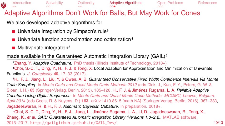
36. Introduction Solvability Optimality Adaptive Algorithms Open Problems References Adaptive Algorithms Don’t Work for Balls, But May Work for Cones We also developed adaptive algorithms for Univariate integration by Simpson’s rule Univariate function approximation and optimization Multivariate integration made available in the Guaranteed Automatic Integration Library (GAIL) Zhang, Y. Adaptive Quadrature. PhD thesis (Illinois Institute of Technology, 2018+). Choi, S.-C. T., Ding, Y., H., F. J. & Tong, X. Local Adaption for Approximation and Minimization of Univariate Functions. J. Complexity 40, 17–33 (2017). H., F. J., Jiang, L., Liu, Y. & Owen, A. B. Guaranteed Conservative Fixed Width Confidence Intervals Via Monte Carlo Sampling. in Monte Carlo and Quasi-Monte Carlo Methods 2012 (eds Dick, J., Kuo, F. Y., Peters, G. W. & Sloan, I. H.) 65 (Springer-Verlag, Berlin, 2013), 105–128, H., F. J. & Jiménez Rugama, L. A. Reliable Adaptive Cubature Using Digital Sequences. in Monte Carlo and Quasi-Monte Carlo Methods: MCQMC, Leuven, Belgium, April 2014 (eds Cools, R. & Nuyens, D.) 163. arXiv:1410.8615 [math.NA] (Springer-Verlag, Berlin, 2016), 367–383, Jagadeeswaran, R. & H., F. J. Automatic Bayesian Cubature. in preparation. 2018+. Choi, S.-C. T., Ding, Y., H., F. J., Jiang, L., Jiménez Rugama, L. A., Li, D., Jagadeeswaran, R., Tong, X., Zhang, K., et al. GAIL: Guaranteed Automatic Integration Library (Versions 1.0–2.2). MATLAB software. 2013–2017. http://gailgithub.github.io/GAIL_Dev/. 10/13
37. Introduction Solvability Optimality Adaptive Algorithms Open Problems References Work to Be Done Find F = for which MATLAB’s integral_g or Chebfun are guaranteed to solve the integration problem Locally adaptive univariate integration Higher order function approximation Adaptive multi-level Monte Carlo methods Adaptive multivariate function approximation Other error criteria, such as relative error or a hybrid of absolute and relative error Combining our software efforts with that of other research groups The MathWorks, Inc. MATLAB 9.5. (Natick, MA, 2018). Hale, N., Trefethen, L. N. & Driscoll, T. A. Chebfun Version 5.7. (2017). Giles, M. Multilevel Monte Carlo Methods. Acta Numer. 24, 259–328 (2015). Ding, Y., H., F. J. & Jiménez Rugama, L. A. An Adaptive Algorithm Employing Continuous Linear Functionals. 2018+. H., F. J., Jiménez Rugama, L. A. & Li, D. in Contemporary Computational Mathematics — a celebration of the 80th birthday of Ian Sloan (eds Dick, J., Kuo, F. Y. & Woźniakowski, H.) 597–619 (Springer-Verlag, 2018). doi:10.1007/978-3-319-72456-0. 11/13
38. Introduction Solvability Optimality Adaptive Algorithms Open Problems References Other Opportunities for You Join the Society for Industrial and Applied Mathematics (SIAM) for free Click here Join the American Statististcal Association (ASA) for $25 per year Click here 12/13
39. Thank you Slides available on SpeakerDeck at speakerdeck.com/fjhickernell/can-we-solve-it-if-so-how-fast
40. Introduction Solvability Optimality Adaptive Algorithms Open Problems References Kunsch, R. J., Novak, E. & Rudolf, D. Solvable Integration Problems and Optimal Sample Size Selection. submitted for publication. 2018+. Clancy, N., Ding, Y., Hamilton, C., H., F. J. & Zhang, Y. The Cost of Deterministic, Adaptive, Automatic Algorithms: Cones, Not Balls. J. Complexity 30, 21–45 (2014). Zhang, Y. Adaptive Quadrature. PhD thesis (Illinois Institute of Technology, 2018+). Choi, S.-C. T., Ding, Y., H., F. J. & Tong, X. Local Adaption for Approximation and Minimization of Univariate Functions. J. Complexity 40, 17–33 (2017). H., F. J., Jiang, L., Liu, Y. & Owen, A. B. Guaranteed Conservative Fixed Width Confidence Intervals Via Monte Carlo Sampling. in Monte Carlo and Quasi-Monte Carlo Methods 2012 (eds Dick, J., Kuo, F. Y., Peters, G. W. & Sloan, I. H.) 65 (Springer-Verlag, Berlin, 2013), 105–128. H., F. J. & Jiménez Rugama, L. A. Reliable Adaptive Cubature Using Digital Sequences. in Monte Carlo and Quasi-Monte Carlo Methods: MCQMC, Leuven, Belgium, April 2014 13/13
41. Introduction Solvability Optimality Adaptive Algorithms Open Problems References (eds Cools, R. & Nuyens, D.) 163. arXiv:1410.8615 [math.NA] (Springer-Verlag, Berlin, 2016), 367–383. Jagadeeswaran, R. & H., F. J. Automatic Bayesian Cubature. in preparation. 2018+. Choi, S.-C. T. et al. GAIL: Guaranteed Automatic Integration Library (Versions 1.0–2.2). MATLAB software. 2013–2017. http://gailgithub.github.io/GAIL_Dev/. The MathWorks, Inc. MATLAB 9.5. (Natick, MA, 2018). Hale, N., Trefethen, L. N. & Driscoll, T. A. Chebfun Version 5.7. (2017). Giles, M. Multilevel Monte Carlo Methods. Acta Numer. 24, 259–328 (2015). Ding, Y., H., F. J. & Jiménez Rugama, L. A. An Adaptive Algorithm Employing Continuous Linear Functionals. 2018+. 13/13
42. Introduction Solvability Optimality Adaptive Algorithms Open Problems References H., F. J., Jiménez Rugama, L. A. & Li, D. in Contemporary Computational Mathematics — a celebration of the 80th birthday of Ian Sloan (eds Dick, J., Kuo, F. Y. & Woźniakowski, H.) 597–619 (Springer-Verlag, 2018). doi:10.1007/978-3-319-72456-0. 13/13