Upgrade to Pro — share decks privately, control downloads, hide ads and more …

Estimating hazardous concentrations for environmental risk assessment with ecotoxicological effect data

Graeme Hickey
December 09, 2008

Estimating hazardous concentrations for environmental risk assessment with ecotoxicological effect data

Presented at the Royal Statistical Society North East Section AGM

Graeme Hickey

December 09, 2008
Tweet

More Decks by Graeme Hickey

Other Decks in Research

Transcript

  1. Outline CRA: Haz. Concs. Loss Functions Salinity SSDs Closing Remarks References
    Estimating Hazardous Concentrations for
    Environmental Risk Assessment with
    Ecotoxicological Effect Data
    Graeme Hickey1 Peter Craig1 Andy Hart2 Ben Kefford3
    Jason Dunlop4
    1Department of Mathematical Sciences, Durham University, UK
    2Central Science Laboratories, York, UK
    3School of Applied Sciences, RMIT, Victoria, Australia
    4Department of Natural Resources and Water, Queensland, Australia
    RSS AGM Meeting, 2008

    View Slide

  2. Outline CRA: Haz. Concs. Loss Functions Salinity SSDs Closing Remarks References
    Outline of presentation:
    1 Background of the risk assessment.
    2 A lower-tier risk assessment problem.
    3 A higher-tier risk assessment problem: an example.

    View Slide

  3. Outline CRA: Haz. Concs. Loss Functions Salinity SSDs Closing Remarks References
    Background
    Background
    I will focus on aquatic Risk Assessment (RA) to chemicals.

    View Slide

  4. Outline CRA: Haz. Concs. Loss Functions Salinity SSDs Closing Remarks References
    Background
    Background
    I will focus on aquatic Risk Assessment (RA) to chemicals.
    Governing bodies (e.g. EU, US-EPA) want to estimate the
    hazardous concentration (HC), i.e. the maximum
    permissible/safe concentration, for a toxicant.

    View Slide

  5. Outline CRA: Haz. Concs. Loss Functions Salinity SSDs Closing Remarks References
    Background
    Background
    I will focus on aquatic Risk Assessment (RA) to chemicals.
    Governing bodies (e.g. EU, US-EPA) want to estimate the
    hazardous concentration (HC), i.e. the maximum
    permissible/safe concentration, for a toxicant.
    The substance might be a discharged chemical (e.g. pesticide
    in a river) or an environmental change (e.g. rising salinity
    toxicity due to land clearing).

    View Slide

  6. Outline CRA: Haz. Concs. Loss Functions Salinity SSDs Closing Remarks References
    Background
    Background
    I will focus on aquatic Risk Assessment (RA) to chemicals.
    Governing bodies (e.g. EU, US-EPA) want to estimate the
    hazardous concentration (HC), i.e. the maximum
    permissible/safe concentration, for a toxicant.
    The substance might be a discharged chemical (e.g. pesticide
    in a river) or an environmental change (e.g. rising salinity
    toxicity due to land clearing).
    For lower-tier RA; if HC < Predicted Environmental
    Concentration then the risk is high. Immediate action required
    or a more refined assessment.

    View Slide

  7. Outline CRA: Haz. Concs. Loss Functions Salinity SSDs Closing Remarks References
    Toxicity Data
    Current (EU) Practice
    0.0 0.4 0.8
    Species 1
    Response
    x1
    0.0 0.4 0.8
    Species 2
    Response
    x2
    and so on...
    0.0 0.4 0.8
    Species n
    Response
    xn
    Toxicity tolerance data for n
    distinct species is provided:
    x1, x2, . . . , xn
    (n is very small!).
    Each xi
    is independently
    derived (estimated) from a
    species dose-response curve,
    which is expensive.
    Experimental error assumed
    negligible, so not propogated.

    View Slide

  8. Outline CRA: Haz. Concs. Loss Functions Salinity SSDs Closing Remarks References
    Current Methods
    Current (EU) Deterministic Approach
    HC def
    = min{x1,x2,...,xn}
    AF

    View Slide

  9. Outline CRA: Haz. Concs. Loss Functions Salinity SSDs Closing Remarks References
    Current Methods
    Current (EU) Deterministic Approach
    HC def
    = min{x1,x2,...,xn}
    AF
    The Assessment Factor (AF) is an arbitrary value (> 1;
    typically 10, 100, or 1000) used to account for uncertainty
    and variability (although not made clear which uncertainties!).
    Concept of risk measurement is replaced with perceived
    conservatism.

    View Slide

  10. Outline CRA: Haz. Concs. Loss Functions Salinity SSDs Closing Remarks References
    Current Methods
    Current Probabilistic Approaches
    Assume y1
    = log(x1
    ), y2
    = log(x2
    ), . . . , yn
    = log(xn
    ) are realisations from
    the same distribution – the Species Sensitivity Distribution (SSD).
    N(µ, σ2) is the typical choice.

    View Slide

  11. Outline CRA: Haz. Concs. Loss Functions Salinity SSDs Closing Remarks References
    Current Methods
    Current Probabilistic Approaches
    Assume y1
    = log(x1
    ), y2
    = log(x2
    ), . . . , yn
    = log(xn
    ) are realisations from
    the same distribution – the Species Sensitivity Distribution (SSD).
    N(µ, σ2) is the typical choice.
    The SSD is defined to be the probability that a randomly selected species
    drawn from the ecological assemblage has its toxicological endpoint
    violated at a specified (log-) environmental concentration.

    View Slide

  12. Outline CRA: Haz. Concs. Loss Functions Salinity SSDs Closing Remarks References
    Current Methods
    Current Probabilistic Approaches
    Assume y1
    = log(x1
    ), y2
    = log(x2
    ), . . . , yn
    = log(xn
    ) are realisations from
    the same distribution – the Species Sensitivity Distribution (SSD).
    N(µ, σ2) is the typical choice.
    The SSD is defined to be the probability that a randomly selected species
    drawn from the ecological assemblage has its toxicological endpoint
    violated at a specified (log-) environmental concentration.
    The HC is often defined to be the p-th percentile of the SSD (HCp
    );
    typically p = 5 based on experience (e.g. Dutch government)

    View Slide

  13. Outline CRA: Haz. Concs. Loss Functions Salinity SSDs Closing Remarks References
    Current Methods
    Current Probabilistic Approaches
    Assume y1
    = log(x1
    ), y2
    = log(x2
    ), . . . , yn
    = log(xn
    ) are realisations from
    the same distribution – the Species Sensitivity Distribution (SSD).
    N(µ, σ2) is the typical choice.
    The SSD is defined to be the probability that a randomly selected species
    drawn from the ecological assemblage has its toxicological endpoint
    violated at a specified (log-) environmental concentration.
    The HC is often defined to be the p-th percentile of the SSD (HCp
    );
    typically p = 5 based on experience (e.g. Dutch government)
    The ‘Gold Standard’ is Aldenberg & Jaworska’s (2000) 50% and lower
    5% confidence limit estimate of the sampling distn 5th percentile –
    estimators are closed form (non-central t).
    Extrapolates whilst accounting for inter-species variability and accounts
    for sampling uncertainty. Ignores other uncertainties!

    View Slide

  14. Outline CRA: Haz. Concs. Loss Functions Salinity SSDs Closing Remarks References
    Current Methods
    A Hypothetical SSD

    View Slide

  15. Outline CRA: Haz. Concs. Loss Functions Salinity SSDs Closing Remarks References
    Connections
    Relation to Loss Functions
    The choice of the lower 5% estimator is prescribed to err on
    the side of caution. But, it has no ecological relevance.

    View Slide

  16. Outline CRA: Haz. Concs. Loss Functions Salinity SSDs Closing Remarks References
    Connections
    Relation to Loss Functions
    The choice of the lower 5% estimator is prescribed to err on
    the side of caution. But, it has no ecological relevance.
    It can be shown that the estimator(s) are Bayes rules w.r.t.
    the class of Generalised Absolute Loss (GAL) functions using
    Jeffreys’ prior: π(µ, σ2) ∝ σ−2 for µ ∈ R, σ2 ∈ R+.; i.e.
    δ∗
    p
    (Y) = arg min
    δ(Y)
    Eµ,σ2|YL ψp(µ, σ2), δ(Y)
    where δ(Y) is an estimator, and ψp(µ, σ2) is the ‘true’
    quantity.

    View Slide

  17. Outline CRA: Haz. Concs. Loss Functions Salinity SSDs Closing Remarks References
    Connections
    −4 −2 0 2 4
    0 10 20 30 40 50 60

    ∆ = δ
    δ −
    − ψ
    ψ
    L(∆
    ∆)
    GAL Function Definition
    L (ψp, δp
    ) =
    C1
    [ψp − δp
    ] if ψp ≥ δp
    C2
    [δp − ψp
    ] if ψp < δp
    for C1 > 0, C2 > 0.

    View Slide

  18. Outline CRA: Haz. Concs. Loss Functions Salinity SSDs Closing Remarks References
    Connections
    −4 −2 0 2 4
    0 10 20 30 40 50 60

    ∆ = δ
    δ −
    − ψ
    ψ
    L(∆
    ∆)
    GAL Function Definition
    L (ψp, δp
    ) =
    C1
    [ψp − δp
    ] if ψp ≥ δp
    C2
    [δp − ψp
    ] if ψp < δp
    for C1 > 0, C2 > 0.
    The percentile choice relates to L
    via C1
    C1+C2
    .

    View Slide

  19. Outline CRA: Haz. Concs. Loss Functions Salinity SSDs Closing Remarks References
    LINEX
    (Modified-) LINEX
    Overestimation of the HCp
    is much more serious than underestimation,
    hence the lower 5th-percentile choice ⇒ asymmetry is a highly desirable
    property.

    View Slide

  20. Outline CRA: Haz. Concs. Loss Functions Salinity SSDs Closing Remarks References
    LINEX
    (Modified-) LINEX
    Overestimation of the HCp
    is much more serious than underestimation,
    hence the lower 5th-percentile choice ⇒ asymmetry is a highly desirable
    property.
    Assuming that a risk manager can specify a loss-benefit portfolio
    independent of their choice of p; we apply an asymmetric & non-linear
    loss function: Zieli´
    nski’s (Modified-) LINear EXponential (LINEX).

    View Slide

  21. Outline CRA: Haz. Concs. Loss Functions Salinity SSDs Closing Remarks References
    LINEX
    (Modified-) LINEX
    Overestimation of the HCp
    is much more serious than underestimation,
    hence the lower 5th-percentile choice ⇒ asymmetry is a highly desirable
    property.
    Assuming that a risk manager can specify a loss-benefit portfolio
    independent of their choice of p; we apply an asymmetric & non-linear
    loss function: Zieli´
    nski’s (Modified-) LINear EXponential (LINEX).

    (δp, ψp
    ) = exp αδp−ψp
    σ
    − α δp−ψp
    σ
    − 1

    View Slide

  22. Outline CRA: Haz. Concs. Loss Functions Salinity SSDs Closing Remarks References
    LINEX
    −4 −2 0 2 4
    0 10 20 30 40


    L(∆
    ∆)
    α
    α=2
    α
    α=0.5
    α
    α=0
    α
    α=1

    View Slide

  23. Outline CRA: Haz. Concs. Loss Functions Salinity SSDs Closing Remarks References
    LINEX
    −4 −2 0 2 4
    0 10 20 30 40


    L(∆
    ∆)
    α
    α=2
    α
    α=0.5
    α
    α=0
    α
    α=1
    Modified-LINEX differs from
    standard case because
    ∆ = δp
    (Y)−ψp
    (µ, σ2) → ∆/σ.

    View Slide

  24. Outline CRA: Haz. Concs. Loss Functions Salinity SSDs Closing Remarks References
    LINEX
    −4 −2 0 2 4
    0 10 20 30 40


    L(∆
    ∆)
    α
    α=2
    α
    α=0.5
    α
    α=0
    α
    α=1
    Modified-LINEX differs from
    standard case because
    ∆ = δp
    (Y)−ψp
    (µ, σ2) → ∆/σ.
    If ∆ was unscaled, the risk
    assessor must have knowledge
    of the SSD slope in advance to
    specify costs/loss (Zieli´
    nski,
    2005).
    Scaling allows the risk manager
    to specify costs on a
    ‘standardised’ scale.

    View Slide

  25. Outline CRA: Haz. Concs. Loss Functions Salinity SSDs Closing Remarks References
    LINEX
    A Decision Rule
    Bayes rules of modified-LINEX and GAL (under Jeffreys’
    prior) is ¯
    y − κpsy , where κp is called an Assessment
    Shift-Factor which is independent of the data.

    View Slide

  26. Outline CRA: Haz. Concs. Loss Functions Salinity SSDs Closing Remarks References
    LINEX
    A Decision Rule
    Bayes rules of modified-LINEX and GAL (under Jeffreys’
    prior) is ¯
    y − κpsy , where κp is called an Assessment
    Shift-Factor which is independent of the data.
    κp =
    a percentile of the non-central t-distribution (GAL);
    scaled parabolic cylinder function (modified-LINEX)
    Allows for tractable, transparent, and fast risk assessment –
    appeals to risk managers.

    View Slide

  27. Outline CRA: Haz. Concs. Loss Functions Salinity SSDs Closing Remarks References
    LINEX
    A Decision Rule
    Bayes rules of modified-LINEX and GAL (under Jeffreys’
    prior) is ¯
    y − κpsy , where κp is called an Assessment
    Shift-Factor which is independent of the data.
    κp =
    a percentile of the non-central t-distribution (GAL);
    scaled parabolic cylinder function (modified-LINEX)
    Allows for tractable, transparent, and fast risk assessment –
    appeals to risk managers.
    We use Jeffreys’ prior to compare to other proposals
    (Aldenberg & Jaworska 2000 and EFSA 2005).

    View Slide

  28. Outline CRA: Haz. Concs. Loss Functions Salinity SSDs Closing Remarks References
    A Comparison
    Comparison of Assessment Shift Factors for HC5
    2 4 6 8 10
    2 5 10 20
    Sample Size
    κ
    κ5 (Assessment Shift Factor)
    LINEX α
    α = 1
    LINEX α
    α = 2
    LINEX α
    α = 3
    A&J γ
    γ = 0.5
    A&J γ
    γ = 0.05
    EFSA

    View Slide

  29. Outline CRA: Haz. Concs. Loss Functions Salinity SSDs Closing Remarks References
    Some Background
    Effects of Salinity
    Salinity levels in Australian aquatic environments are
    increasing, due to poor management practices.
    A lot of time and resources has been spent on researching
    agricultural and economic effects.

    View Slide

  30. Outline CRA: Haz. Concs. Loss Functions Salinity SSDs Closing Remarks References
    Some Background
    It’s Predicted To Get Worse...
    Year: 2000
    Area at Risk = 5,658,000 Ha

    View Slide

  31. Outline CRA: Haz. Concs. Loss Functions Salinity SSDs Closing Remarks References
    Some Background
    It’s Predicted To Get Worse...
    Year: 2000
    Area at Risk = 5,658,000 Ha
    Year: 2050
    Area at Risk = 17,000,000 Ha

    View Slide

  32. Outline CRA: Haz. Concs. Loss Functions Salinity SSDs Closing Remarks References
    Remodelling
    Beginning of a New Model
    Salinity risk assessment is high stakes! This requires a higher
    level RA.

    View Slide

  33. Outline CRA: Haz. Concs. Loss Functions Salinity SSDs Closing Remarks References
    Remodelling
    Beginning of a New Model
    Salinity risk assessment is high stakes! This requires a higher
    level RA.
    In high enough concentrations, it’s toxic to freshwater species.

    View Slide

  34. Outline CRA: Haz. Concs. Loss Functions Salinity SSDs Closing Remarks References
    Remodelling
    Beginning of a New Model
    Salinity risk assessment is high stakes! This requires a higher
    level RA.
    In high enough concentrations, it’s toxic to freshwater species.
    A new and more efficient experimental technique has been
    proposed by Kefford et al. (2005).

    View Slide

  35. Outline CRA: Haz. Concs. Loss Functions Salinity SSDs Closing Remarks References
    Remodelling
    Beginning of a New Model
    Salinity risk assessment is high stakes! This requires a higher
    level RA.
    In high enough concentrations, it’s toxic to freshwater species.
    A new and more efficient experimental technique has been
    proposed by Kefford et al. (2005).
    We get: (i) more toxicity data; and (ii) in better proportion to
    ecological structure.

    View Slide

  36. Outline CRA: Haz. Concs. Loss Functions Salinity SSDs Closing Remarks References
    Remodelling
    Beginning of a New Model
    Salinity risk assessment is high stakes! This requires a higher
    level RA.
    In high enough concentrations, it’s toxic to freshwater species.
    A new and more efficient experimental technique has been
    proposed by Kefford et al. (2005).
    We get: (i) more toxicity data; and (ii) in better proportion to
    ecological structure.
    With more data, we can use more complicated modelling of
    the SSD; e.g. O’Hagan (2005).

    View Slide

  37. Outline CRA: Haz. Concs. Loss Functions Salinity SSDs Closing Remarks References
    Remodelling
    Beginning of a New Model
    Salinity risk assessment is high stakes! This requires a higher
    level RA.
    In high enough concentrations, it’s toxic to freshwater species.
    A new and more efficient experimental technique has been
    proposed by Kefford et al. (2005).
    We get: (i) more toxicity data; and (ii) in better proportion to
    ecological structure.
    With more data, we can use more complicated modelling of
    the SSD; e.g. O’Hagan (2005).
    We are interested in the Victorian environment.

    View Slide

  38. Outline CRA: Haz. Concs. Loss Functions Salinity SSDs Closing Remarks References
    Results
    Current SSD Handling
    0 20 40 60 80
    0.0 0.2 0.4 0.6 0.8 1.0
    Concentration mS/cm
    Probability of Survival
    New technique prescribes many (doubly) censored toxicity
    values – wasteful to discard (c.f. current regulatory policies)

    View Slide

  39. Outline CRA: Haz. Concs. Loss Functions Salinity SSDs Closing Remarks References
    Remodelling
    Beginning of a New Model
    Model 1: Bayesian Extension of Aldenberg & Jaworska (2000)
    yi ∼ N(µ, σ2)
    ⇒ FSSD
    (y) = Φ y−µ
    σ

    View Slide

  40. Outline CRA: Haz. Concs. Loss Functions Salinity SSDs Closing Remarks References
    Remodelling
    Beginning of a New Model
    Model 1: Bayesian Extension of Aldenberg & Jaworska (2000)
    yi ∼ N(µ, σ2)
    ⇒ FSSD
    (y) = Φ y−µ
    σ
    Model 2: A Version of O’Hagan et al.
    yi ∼ N(µti
    , σ2) where ti
    = taxonomic order of species i.
    ⇒ FSSD
    (y) = N
    t=1
    ωt
    Φ y−µt
    σ
    where ωt
    are the ‘estimated’ (or
    otherwise) taxonomic order weights.

    View Slide

  41. Outline CRA: Haz. Concs. Loss Functions Salinity SSDs Closing Remarks References
    Remodelling
    Beginning of a New Model
    Model 1: Bayesian Extension of Aldenberg & Jaworska (2000)
    yi ∼ N(µ, σ2)
    ⇒ FSSD
    (y) = Φ y−µ
    σ
    Model 2: A Version of O’Hagan et al.
    yi ∼ N(µti
    , σ2) where ti
    = taxonomic order of species i.
    ⇒ FSSD
    (y) = N
    t=1
    ωt
    Φ y−µt
    σ
    where ωt
    are the ‘estimated’ (or
    otherwise) taxonomic order weights.
    Prior Distributions
    Expert elicitations for µt
    ’s.
    All other parameters – applied posterior distributions updated with
    (training data) Queensland data.

    View Slide

  42. Outline CRA: Haz. Concs. Loss Functions Salinity SSDs Closing Remarks References
    Results
    Posterior SSD(s) / HC5
    (s) for Model 1
    5 10 20 50 100 200
    0.0 0.2 0.4 0.6 0.8 1.0
    Concentration mS/cm
    Cumulative Probability
    q
    q
    q
    q
    q
    q
    q
    q
    q
    q
    q
    q
    q
    q
    q
    q
    q
    q
    q
    q
    q
    q
    q
    q
    q
    q
    q
    q
    q
    q
    q
    q
    q
    q
    q
    q
    q
    q
    q
    q
    q
    q
    q
    q
    q
    q
    q
    q
    8 10 12 14
    0.0 0.2 0.4 0.6 0.8 1.0
    HC5 mS/cm
    Cumulative Probability

    View Slide

  43. Outline CRA: Haz. Concs. Loss Functions Salinity SSDs Closing Remarks References
    Results
    Posterior SSDs / HC5
    s for Model 2
    Case (i) estimated values of ωi .
    Case (ii) all orders equal (ωi = ωj ).
    Case (iii) estimated values for 6 most dense orders (scaled)
    5 10 20 50 100 200
    0.0 0.2 0.4 0.6 0.8 1.0
    Concentration mS/cm
    Cumulative Probability
    q
    q
    q
    q
    q
    q
    q
    q
    q
    q
    q
    q
    q
    q
    q
    q
    q
    q
    q
    q
    q
    q
    q
    q
    q
    q
    q
    q
    q
    q
    q
    q
    q
    q
    q
    q
    q
    q
    q
    q
    q
    q
    q
    q
    q
    q
    q
    q
    Case (i)
    Case (ii)
    Case (iii)
    4 6 8 10 12 14 16
    0.0 0.2 0.4 0.6 0.8 1.0
    HC5 mS/cm
    Cumulative Probability
    Case (i)
    Case (ii)
    Case (iii)

    View Slide

  44. Outline CRA: Haz. Concs. Loss Functions Salinity SSDs Closing Remarks References
    Discussion & Conclusions
    Current probabilistic proposals for estimating the HC and risk are based
    on arbitrary or unsatisfactory principles, as demonstrated by reducing
    them to loss functions.

    View Slide

  45. Outline CRA: Haz. Concs. Loss Functions Salinity SSDs Closing Remarks References
    Discussion & Conclusions
    Current probabilistic proposals for estimating the HC and risk are based
    on arbitrary or unsatisfactory principles, as demonstrated by reducing
    them to loss functions.
    EU Technical Guidance Document allows for probabilistic application of
    SSD based estimators (although not clear how) – so there is motivation
    for development.

    View Slide

  46. Outline CRA: Haz. Concs. Loss Functions Salinity SSDs Closing Remarks References
    Discussion & Conclusions
    Current probabilistic proposals for estimating the HC and risk are based
    on arbitrary or unsatisfactory principles, as demonstrated by reducing
    them to loss functions.
    EU Technical Guidance Document allows for probabilistic application of
    SSD based estimators (although not clear how) – so there is motivation
    for development.
    The extrapolation methods discussed [here] only account for natural
    species variability and sampling uncertainty. There are other uncertainties
    – lots of them! Does over-conservatism allow us to mask these additional
    uncertainties? Answer: We don’t know (yet!).

    View Slide

  47. Outline CRA: Haz. Concs. Loss Functions Salinity SSDs Closing Remarks References
    Discussion & Conclusions
    Current probabilistic proposals for estimating the HC and risk are based
    on arbitrary or unsatisfactory principles, as demonstrated by reducing
    them to loss functions.
    EU Technical Guidance Document allows for probabilistic application of
    SSD based estimators (although not clear how) – so there is motivation
    for development.
    The extrapolation methods discussed [here] only account for natural
    species variability and sampling uncertainty. There are other uncertainties
    – lots of them! Does over-conservatism allow us to mask these additional
    uncertainties? Answer: We don’t know (yet!).
    Restrictions to data impoverishment should be addressed; c.f. Kefford et
    al.’s technique.

    View Slide

  48. Outline CRA: Haz. Concs. Loss Functions Salinity SSDs Closing Remarks References
    Discussion & Conclusions
    Current probabilistic proposals for estimating the HC and risk are based
    on arbitrary or unsatisfactory principles, as demonstrated by reducing
    them to loss functions.
    EU Technical Guidance Document allows for probabilistic application of
    SSD based estimators (although not clear how) – so there is motivation
    for development.
    The extrapolation methods discussed [here] only account for natural
    species variability and sampling uncertainty. There are other uncertainties
    – lots of them! Does over-conservatism allow us to mask these additional
    uncertainties? Answer: We don’t know (yet!).
    Restrictions to data impoverishment should be addressed; c.f. Kefford et
    al.’s technique.
    We can invert the risk assessment problem to answer: How do we
    prioritise clean-up operations with finite resources?

    View Slide

  49. Outline CRA: Haz. Concs. Loss Functions Salinity SSDs Closing Remarks 
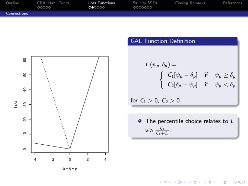
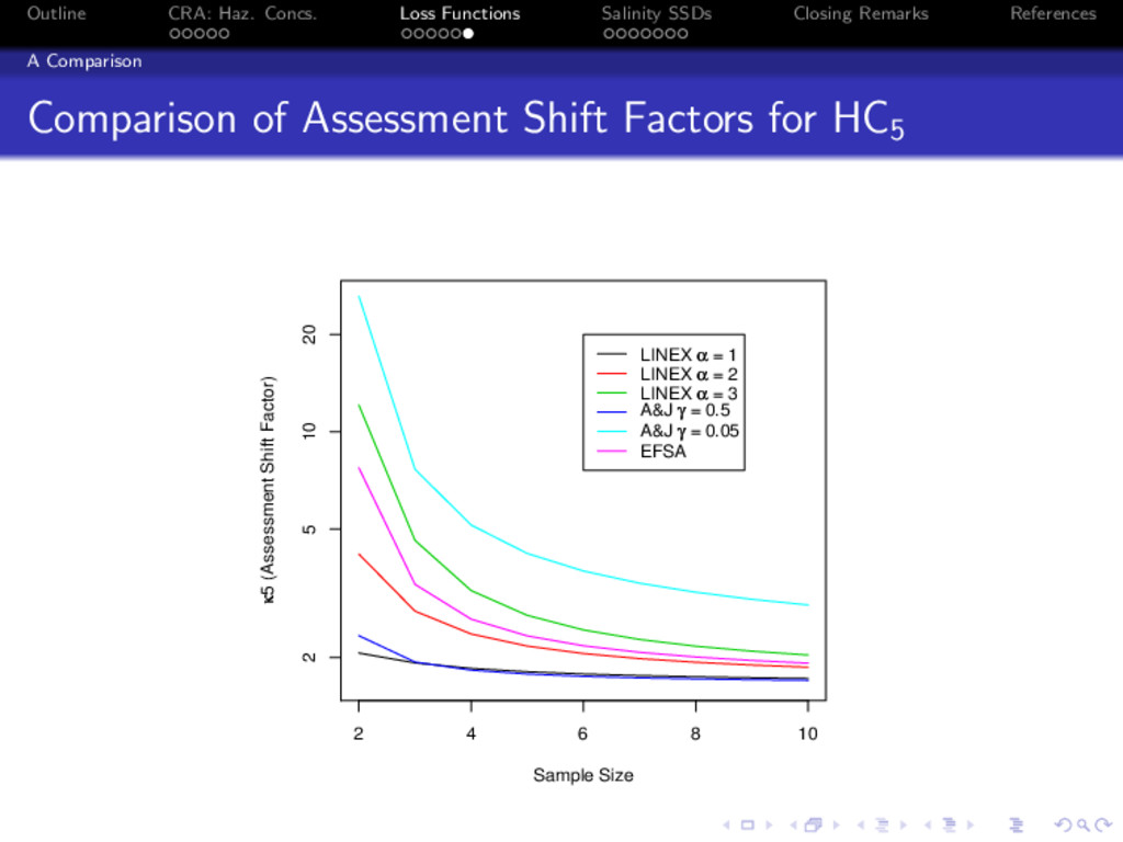
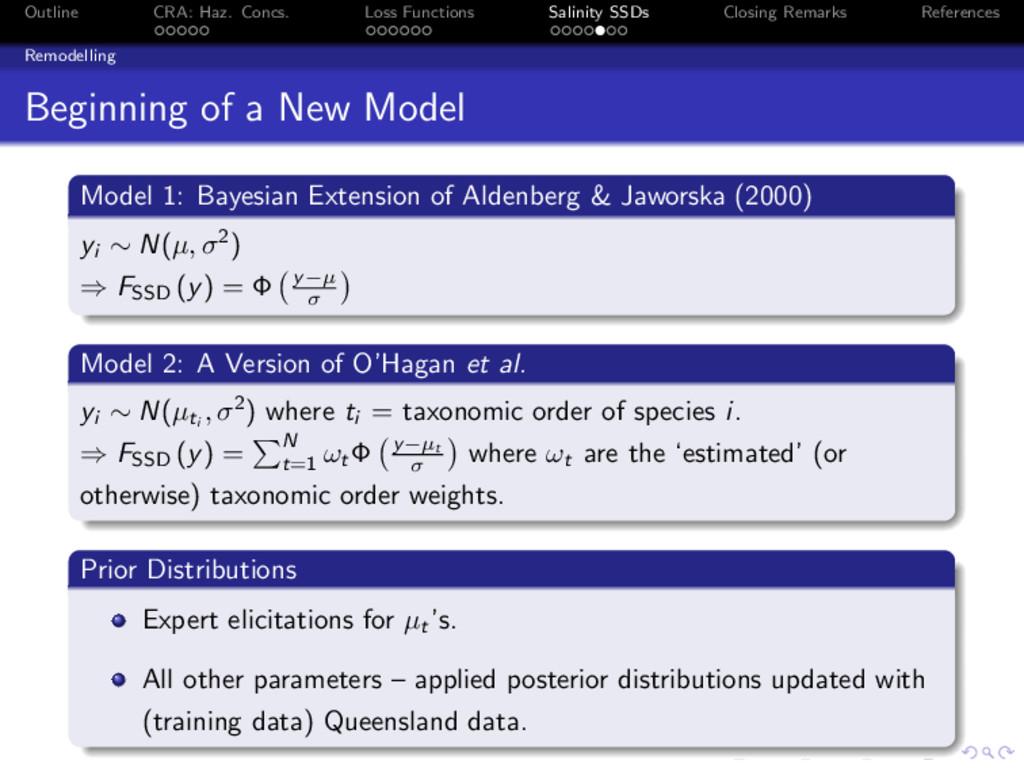
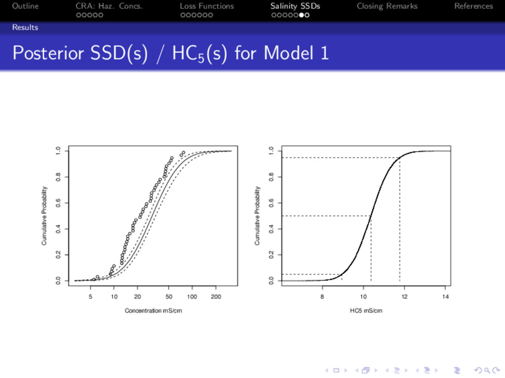
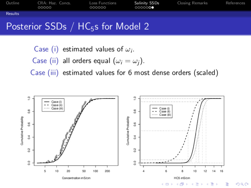
References
    References
    Aldenberg, T. and Jaworska, J. S. (2000). Uncertainty of the Hazardous Concentration and Fraction
    Affected for Normal Species Sensitivity Distributions. Ecotoxicol. Environ. Saf. 46, 1–18.
    European Food Safety Authority Panel on Plant Health, Plant Protection Products and their Residues
    (2005). Question No. EFSA-Q-2005-042. The EFSA Journal. 301, 1–45.
    Hickey, G. L., Kefford, B. J., Dunlop, J. E. and Craig, P. S. (2008). Making Species Salinity Sensitivity
    Distributions Reflective of Naturally Occurring Communities: Using Rapid Testing and Bayesian Statistics.
    Environ. Toxicol. Chem. 27, No. 11, pp. 2403–2411.
    Hickey, G. L., Craig, P. S. and Hart, A. (2009). On The Application of Loss Functions in Determining
    Assessment Factors for Ecological Risk. Ecotoxicol. Environ. Saf. 72, No. 2, pp. 293–300.
    O’Hagan, A., Crane, M., Grist, E. P. M. and Whitehouse, P. (2005). Estimating Species Sensitivity
    Distributions With the Aid of Expert Judgements. Unpublished.
    http://www.tonyohagan.co.uk/academic/pdf/SSD-stat.pdf
    Zieli´
    nski, R. (2005). Estimating Quantiles With Linex Loss Function. Applications to VaR Estimation.
    Applicationes Mathematicae. 32: 367–373.

    View Slide