Modeling Social Data, Lecture 12: Causality and Experiments

Transcript

1. Causality & Experiments MODELING SOCIAL DATA JAKE HOFMAN COLUMBIA UNIVERSITY
2. Prediction Seeing: Make a forecast, leaving the world as it is vs. Causation Doing: Anticipate what will happen when you make a change in the world
3. Prediction Seeing: Make a forecast, leaving the world as it is (seeing my neighbor with an umbrella might predict rain) vs. Causation Doing: Anticipate what will happen when you make a change in the world (but handing my neighbor an umbrella doesn’t cause rain)
4. “Causes of effects” It’s tempting to ask “what caused Y”, e.g. ◦ What makes an email spam? ◦ What caused my kid to get sick? ◦ Why did the stock market drop? This is ”reverse causal inference”, and is generally quite hard John Stuart Mill (1843)
5. “Effects of causes” Alternatively, we can ask “what happens if we do X?”, e.g. ◦ How does education impact future earnings? ◦ What is the effect of advertising on sales? ◦ How does hospitalization affect health? This is “forward causal inference”: still hard, but less contentious! John Stuart Mill (1843)
6. Example: Hospitalization on health What’s wrong with estimating this model from observational data? Health tomorrow Hospital visit today Effect? Arrow means “X causes Y”
7. Confounds The effect and cause might be confounded by a common cause, and be changing together as a result Health tomorrow Hospital visit today Effect? Health today Dashed circle means “unobserved”
8. Confounds If we only get to observe them changing together, we can’t estimate the effect of hospitalization changing alone Health tomorrow Hospital visit today Effect? Health today
9. A counterfactual (what-if) definition What if you would have acted differently? E.g., how does the health of a hospitalized patient compare to their health if they would have stayed home? We only get to observe one of these outcomes, which is the fundamental problem of causal inference How does this differ from an observational estimate?
10. Observational estimates Let’s say all sick people in our dataset went to the hospital today, and healthy people stayed home The observed difference in health tomorrow is: Δobs = (Sick and went to hospital) – (Healthy and stayed home)
11. Observational estimates Let’s say all sick people in our dataset went to the hospital today, and healthy people stayed home The observed difference in health tomorrow is: Δobs = [(Sick and went to hospital) – (Sick if stayed home)] + [(Sick if stayed home) - (Healthy and stayed home)]
12. Selection bias Let’s say all sick people in our dataset went to the hospital today, and healthy people stayed home The observed difference in health tomorrow is: Δobs = [(Sick and went to hospital) – (Sick if stayed home)] + [(Sick if stayed home) - (Healthy and stayed home)] Causal effect Selection bias (Baseline difference between those who opted in to the treatment and those who didn’t)
13. Basic identity of causal inference Let’s say all sick people in our dataset went to the hospital today, and healthy people stayed home The observed difference in health tomorrow is: Observed difference = Causal effect – Selection bias Selection bias is likely negative here, making the observed difference an underestimate of the causal effect
14. Simpson’s paradox Selection bias can be so large that observational and causal estimates give opposite effects (e.g., going to hospitals makes you less healthy) http://vudlab.com/simpsons
15. Simpson’s paradox So which is right, the aggregated or the partitioned? It depends on the causal mechanism https://en.wikipedia.org/wiki/Simpson%27s_paradox
16. Simpson’s paradox So which is right, the aggregated or the partitioned? It depends on the causal mechanism Morgan and Winship (2015) 108 Chapter 4. Models of Causal Exposure and Identification Criteria Motivation SAT Rejected Admitted Applicants to a Hypothetical College Figure 4.2 Simulation of conditional dependence within values of a collider variable.
17. “To find out what happens when you change something, it is necessary to change it.” -GEORGE BOX
18. Controlled experiments
19. Counterfactuals To isolate the causal effect, we have to change one and only one thing (hospital visits), and compare outcomes + vs (what happened) Reality (what would have happened) Counterfactual
20. The ideal causal estimate CLONE EACH PERSON SEND ONE COPY TO THE HOSPITAL, MAKE THE OTHER STAY HOME MEASURE THE DIFFERENCE IN HEALTH BETWEEN THE COPIES
21. But this might be confounded for various reasons---e.g., Mark has a different diet than Scott
22. Counterfactuals We never get to observe what would have happened if we did something else, so we have to estimate it + vs (what happened) Reality (what would have happened) Counterfactual
23. Random assignment We can use randomization to create two groups that differ only in which treatment they receive, restoring symmetry + World 1 World 2 Heads Tails
24. Random assignment We can use randomization to create two groups that differ only in which treatment they receive, restoring symmetry + World 1 World 2 Heads Tails
25. Random assignment We can use randomization to create two groups that differ only in which treatment they receive, restoring symmetry + World 1 World 2
26. Basic identity of causal inference The observed difference is now the causal effect: Observed difference = Causal effect – Selection bias = Causal effect Selection bias is zero, since there’s no difference, on average, between those who were hospitalized and those who weren’t
27. Hospital visit today Random assignment Random assignment determines the treatment independent of any confounds Health tomorrow Effect? Health today Coin flip Double lines mean “intervention”
28. Random assignment Dunning (2012)
29. Experiments: Caveats / limitations Random assignment is the “gold standard” for causal inference, but it has some limitations: ◦ Randomization often isn’t feasible and/or ethical ◦ Experiments are costly in terms of time and money ◦ It’s difficult to create convincing parallel worlds ◦ Effects in the lab can differ from real-world effects ◦ Inevitably people deviate from their random assignments
30. Validity of experiments INTERNAL VALIDITY Could anything other than the treatment (i.e. a confound) have produced this outcome? Was the study double-blind? Did doctors give the experimental drug to some especially sick patients (breaking randomization) hoping that it would save them? Or treat patients differently based on whether they got the drug or not? EXTERNAL VALIDITY Do the results of the experiment hold in settings we care about? Would this medication be just as effective outside of a clinical trial, when usage is less rigorously monitored or when tried on a different population of patients? Slide thanks to Andrew Mao
31. Expanding the experiment design space Complexity, Realism Size, Scale Duration, Participation Physical labs • Longer periods of time • Fewer constraints on location • More samples of data • Large-scale social interaction • Realistic vs. abstract, simple tasks • More precise instrumentation A software-based “virtual lab” with online participants Slide thanks to Andrew Mao
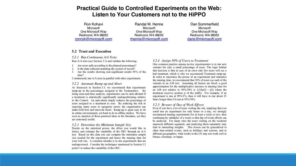
32. personal use. Not for redistribution. The definitive version is published in KDD 2007 (http://www.kdd2007.com/) Practical Guide to Controlled Experiments on the Web: Listen to Your Customers not to the HiPPO Ron Kohavi Microsoft One Microsoft Way Redmond, WA 98052 ronnyk@microsoft.com Randal M. 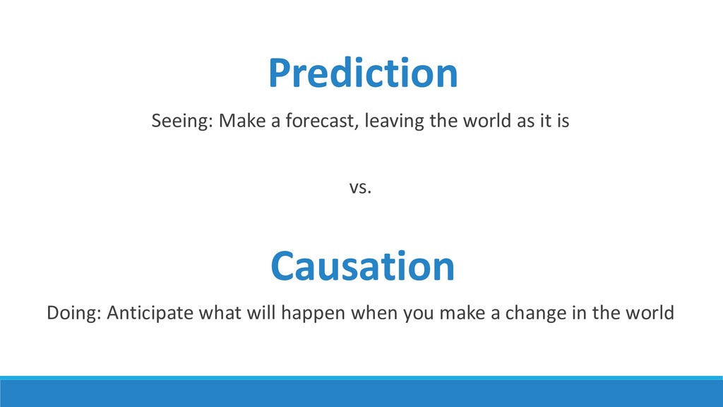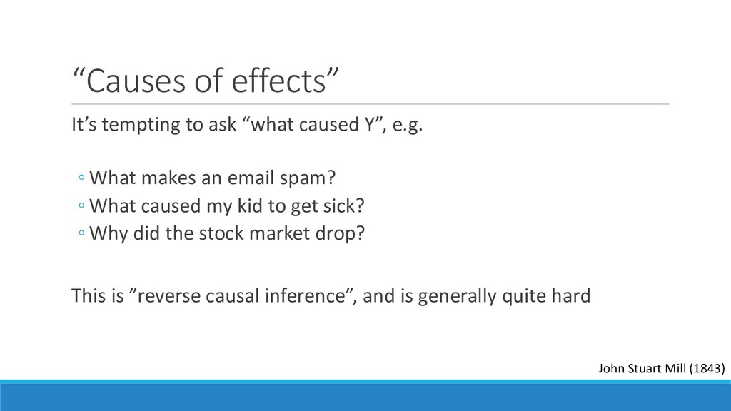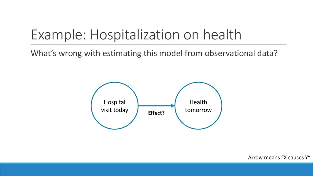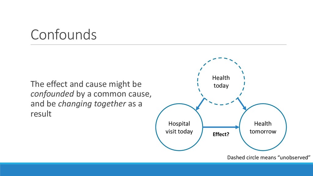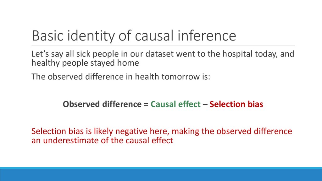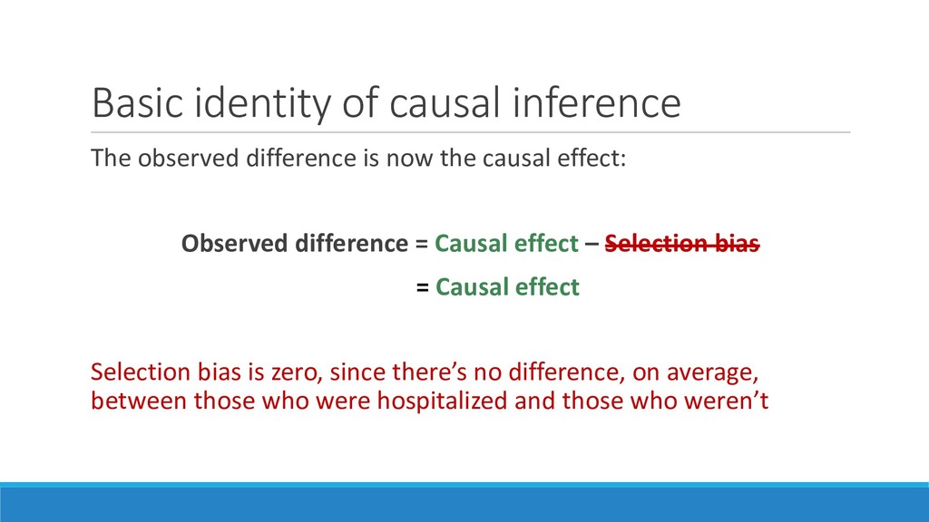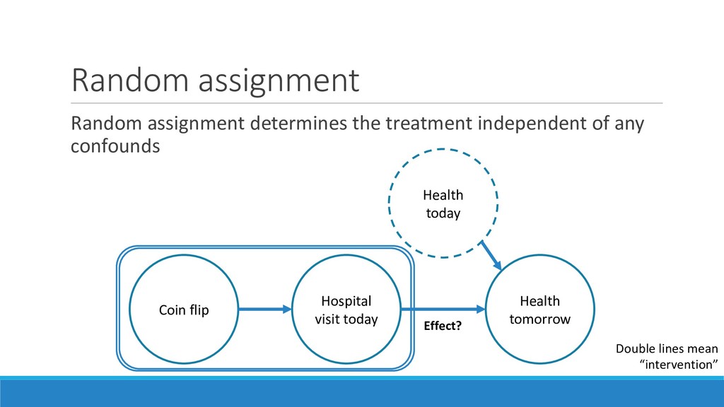Henne Microsoft One Microsoft Way Redmond, WA 98052 rhenne@microsoft.com Dan Sommerfield Microsoft One Microsoft Way Redmond, WA 98052 dans@microsoft.com ABSTRACT The web provides an unprecedented opportunity to evaluate ideas quickly using controlled experiments, also called randomized experiments (single-factor or factorial designs), A/B tests (and their generalizations), split tests, Control/Treatment tests, and parallel flights. Controlled experiments embody the best scientific design for establishing a causal relationship between changes and their influence on user-observable behavior. We provide a practical guide to conducting online experiments, where end-users can help guide the development of features. Our experience indicates that significant learning and return-on- investment (ROI) are seen when development teams listen to their customers, not to the Highest Paid Person’s Opinion (HiPPO). We provide several examples of controlled experiments with surprising results. We review the important ingredients of running controlled experiments, and discuss their limitations (both technical and organizational). We focus on several areas that are critical to experimentation, including statistical power, sample size, and techniques for variance reduction. We describe common architectures for experimentation systems and analyze their advantages and disadvantages. We evaluate randomization and hashing techniques, which we show are not as simple in practice as is often assumed. Controlled experiments typically generate large amounts of data, which can be analyzed using data mining techniques to gain deeper understanding of the factors influencing the outcome of interest, leading to new hypotheses and creating a virtuous cycle of improvements. Organizations that embrace controlled experiments with clear evaluation criteria can evolve their systems with automated optimizations and real-time analyses. Based on our extensive practical experience with multiple systems and organizations, we share key lessons that will help practitioners in running trustworthy controlled experiments. Categories and Subject Descriptors G.3 Probability and Statistics/Experimental Design: controlled experiments, randomized experiments, A/B testing. I.2.6 Learning: real-time, automation, causality. 1. INTRODUCTION One accurate measurement is worth more than a thousand expert opinions — Admiral Grace Hopper In the 1700s, a British ship’s captain observed the lack of scurvy among sailors serving on the naval ships of Mediterranean countries, where citrus fruit was part of their rations. He then gave half his crew limes (the Treatment group) while the other half (the Control group) continued with their regular diet. Despite much grumbling among the crew in the Treatment group, the experiment was a success, showing that consuming limes prevented scurvy. While the captain did not realize that scurvy is a consequence of vitamin C deficiency, and that limes are rich in vitamin C, the intervention worked. British sailors eventually were compelled to consume citrus fruit regularly, a practice that gave rise to the still-popular label limeys (1). Some 300 years later, Greg Linden at Amazon created a prototype to show personalized recommendations based on items in the shopping cart (2). You add an item, recommendations show up; add another item, different recommendations show up. Linden notes that while the prototype looked promising, ―a marketing senior vice-president was dead set against it,‖ claiming it will distract people from checking out. Greg was ―forbidden to work on this any further.‖ Nonetheless, Greg ran a controlled experiment, and the ―feature won by such a wide margin that not having it live was costing Amazon a noticeable chunk of change. With new urgency, shopping cart recommendations launched.‖ Since then, multiple sites have copied cart recommendations. The authors of this paper were involved in many experiments at Amazon, Microsoft, Dupont, and NASA. The culture of experimentation at Amazon, where data trumps intuition (3), and a system that made running experiments easy, allowed Amazon to innovate quickly and effectively. At Microsoft, there are multiple systems for running controlled experiments. We describe several — Jan L.A. van de Snepscheut eoretical techniques seem well suited for practical use and ire significant ingenuity to apply them to messy real world ments. Controlled experiments are no exception. Having rge number of online experiments, we now share several l lessons in three areas: (i) analysis; (ii) trust and on; and (iii) culture and business. Analysis Mine the Data olled experiment provides more than just a single bit of tion about whether the difference in OECs is statistically ant. Rich data is typically collected that can be analyzed achine learning and data mining techniques. For example, riment showed no significant difference overall, but a on of users with a specific browser version was antly worse for the Treatment. The specific Treatment which involved JavaScript, was buggy for that browser and users abandoned. Excluding the population from the showed positive results, and once the bug was fixed, the was indeed retested and was positive. Speed Matters ment might provide a worse user experience because of its ance. Greg Linden (36 p. 15) wrote that experiments at n showed a 1% sales decrease for an additional 100msec, t a specific experiments at Google, which increased the display search results by 500 msecs reduced revenues by ased on a talk by Marissa Mayer at Web 2.0). If time is ctly part of your OEC, make sure that a new feature that is s not losing because it is slower. Test One Factor at a Time (or Not) authors (19 p. 76; 20) recommend testing one factor at a We believe the advice, interpreted narrowly, is too ve and can lead organizations to focus on small 5.2 Trust and Execution 5.2.1 Run Continuous A/A Tests Run A/A tests (see Section 3.1) and validate the following. 1. Are users split according to the planned percentages? 2. Is the data collected matching the system of record? 3. Are the results showing non-significant results 95% of the time? Continuously run A/A tests in parallel with other experiments. 5.2.2 Automate Ramp-up and Abort As discussed in Section 3.3, we recommend that experiments ramp-up in the percentages assigned to the Treatment(s). By doing near-real-time analysis, experiments can be auto-aborted if a treatment is statistically significantly underperforming relative to the Control. An auto-abort simply reduces the percentage of users assigned to a treatment to zero. By reducing the risk in exposing many users to egregious errors, the organization can make bold bets and innovate faster. Ramp-up is quite easy to do in online environments, yet hard to do in offline studies. We have seen no mention of these practical ideas in the literature, yet they are extremely useful. 5.2.3 Determine the Minimum Sample Size Decide on the statistical power, the effect you would like to detect, and estimate the variability of the OEC through an A/A test. Based on this data you can compute the minimum sample size needed for the experiment and hence the running time for your web site. A common mistake is to run experiments that are underpowered. Consider the techniques mentioned in Section 3.2 point 3 to reduce the variability of the OEC. 5.2.4 Assign 50% of Users to Treatment One common practice among novice experimenters is to run new variants for only a small percentage of users. The logic behind that decision is that in case of an error only few users will see a http://exp-platform.com/hippo.aspx Page 7 significant. Rich data is typically collected that can be analyzed using machine learning and data mining techniques. For example, an experiment showed no significant difference overall, but a population of users with a specific browser version was significantly worse for the Treatment. The specific Treatment feature, which involved JavaScript, was buggy for that browser version and users abandoned. Excluding the population from the analysis showed positive results, and once the bug was fixed, the feature was indeed retested and was positive. 5.1.2 Speed Matters A Treatment might provide a worse user experience because of its performance. Greg Linden (36 p. 15) wrote that experiments at Amazon showed a 1% sales decrease for an additional 100msec, and that a specific experiments at Google, which increased the time to display search results by 500 msecs reduced revenues by 20% (based on a talk by Marissa Mayer at Web 2.0). If time is not directly part of your OEC, make sure that a new feature that is losing is not losing because it is slower. 5.1.3 Test One Factor at a Time (or Not) Several authors (19 p. 76; 20) recommend testing one factor at a time. We believe the advice, interpreted narrowly, is too restrictive and can lead organizations to focus on small incremental improvements. Conversely, some companies are touting their fractional factorial designs and Taguchi methods, thus introducing complexity where it may not be needed. While it is clear that factorial designs allow for joint optimization of factors, and are therefore superior in theory (15; 16) our experience from running experiments in online web sites is that interactions are less frequent than people assume (33), and awareness of the issue is enough that parallel interacting experiments are avoided. Our recommendations are therefore: x Conduct single-factor experiments for gaining insights and when you make incremental changes that could be decoupled. x Try some bold bets and very different designs. For example, let two designers come up with two very different designs for a new feature and try them one against the other. You might then start to perturb the winning version to improve it further. For backend algorithms it is even easier to try a completely different algorithm (e.g., a new recommendation algorithm). Data mining can help isolate areas where the new algorithm is significantly better, leading to interesting insights. x Use factorial designs when several factors are suspected to interact strongly. Limit the factors and the possible values per factor because users will be fragmented (reducing power) and because testing the combinations for launch is hard. doing near-real-time analysis, experiments can be auto-aborted if a treatment is statistically significantly underperforming relative to the Control. An auto-abort simply reduces the percentage of users assigned to a treatment to zero. By reducing the risk in exposing many users to egregious errors, the organization can make bold bets and innovate faster. Ramp-up is quite easy to do in online environments, yet hard to do in offline studies. We have seen no mention of these practical ideas in the literature, yet they are extremely useful. 5.2.3 Determine the Minimum Sample Size Decide on the statistical power, the effect you would like to detect, and estimate the variability of the OEC through an A/A test. Based on this data you can compute the minimum sample size needed for the experiment and hence the running time for your web site. A common mistake is to run experiments that are underpowered. Consider the techniques mentioned in Section 3.2 point 3 to reduce the variability of the OEC. 5.2.4 Assign 50% of Users to Treatment One common practice among novice experimenters is to run new variants for only a small percentage of users. The logic behind that decision is that in case of an error only few users will see a bad treatment, which is why we recommend Treatment ramp-up. In order to maximize the power of an experiment and minimize the running time, we recommend that 50% of users see each of the variants in an A/B test. Assuming all factors are fixed, a good approximation for the multiplicative increase in running time for an A/B test relative to 50%/50% is 1/(4 1 − ) where the treatment receives portion of the traffic. For example, if an experiment is run at 99%/1%, then it will have to run about 25 times longer than if it ran at 50%/50%. 5.2.5 Beware of Day of Week Effects Even if you have a lot of users visiting the site, implying that you could run an experiment for only hours or a day, we strongly recommend running experiments for at least a week or two, then continuing by multiples of a week so that day-of-week effects can be analyzed. For many sites the users visiting on the weekend represent different segments, and analyzing them separately may lead to interesting insights. This lesson can be generalized to other time-related events, such as holidays and seasons, and to different geographies: what works in the US may not work well in France, Germany, or Japan. Putting 5.2.3, 5.2.4, and 5.2.5 together, suppose that the power calculations imply that you need to run an A/B test for a minimum of 5 days, if the experiment were run at 50%/50%. We would
33. Experimental evidence of massive-scale emotional contagion through social networks Adam D. I. Kramera,1, Jamie E. Guilloryb,2, and Jeffrey T. Hancockb,c aCore Data Science Team, Facebook, Inc., Menlo Park, CA 94025; and Departments of bCommunication and cInformation Science, Cornell University, Ithaca, NY 14853 Edited by Susan T. Fiske, Princeton University, Princeton, NJ, and approved March 25, 2014 (received for review October 23, 2013) Emotional states can be transferred to others via emotional contagion, leading people to experience the same emotions without their awareness. Emotional contagion is well established in laboratory experiments, with people transferring positive and negative emotions to others. Data from a large real-world social network, collected over a 20-y period suggests that longer-lasting moods (e.g., depression, happiness) can be transferred through networks [Fowler JH, Christakis NA (2008) BMJ 337:a2338], al- though the results are controversial. In an experiment with people who use Facebook, we test whether emotional contagion occurs outside of in-person interaction between individuals by reducing the amount of emotional content in the News Feed. When positive expressions were reduced, people produced fewer positive posts and more negative posts; when negative expressions were re- duced, the opposite pattern occurred. These results indicate that emotions expressed by others on Facebook influence our own emotions, constituting experimental evidence for massive-scale contagion via social networks. This work also suggests that, in contrast to prevailing assumptions, in-person interaction and non- verbal cues are not strictly necessary for emotional contagion, and demonstrated that (i) emotional contagion occurs via text-based computer-mediated communication (7); (ii) contagion of psy- chological and physiological qualities has been suggested based on correlational data for social networks generally (7, 8); and (iii) people’s emotional expressions on Facebook predict friends’ emotional expressions, even days later (7) (although some shared experiences may in fact last several days). To date, however, there is no experimental evidence that emotions or moods are contagious in the absence of direct interaction between experiencer and target. On Facebook, people frequently express emotions, which are later seen by their friends via Facebook’s “News Feed” product (8). Because people’s friends frequently produce much more content than one person can view, the News Feed filters posts, stories, and activities undertaken by friends. News Feed is the primary manner by which people see content that friends share. Which content is shown or omitted in the News Feed is de- termined via a ranking algorithm that Facebook continually develops and tests in the interest of showing viewers the content they will find most relevant and engaging. One such test is reported in this study: A test of whether posts with emotional ed to others via emotional ence the same emotions as agion is well established in people transfer positive and hers. Similarly, data from llected over a 20-y period e.g., depression, happiness) as well (2, 3). effect as contagion of mood tudy’s correlational nature, ion of contextual variables eriences (4, 5), raising im- n processes in networks. An this scrutiny directly; how- periments have been criti- cial interactions. Interacting d an unhappy person, un- esult from experiencing an a partner’s emotion. Prior whether nonverbal cues are f verbal cues alone suffice. e moods are correlated in s possible, but the causal sses occur for emotions in sive in the absence of ex- rs have suggested that in posure to emotional content led people to post content that was consistent with the exposure—thereby testing whether exposure to verbal affective expressions leads to similar verbal expressions, a form of emotional contagion. People who viewed Facebook in English were qualified for selection into the experiment. Two parallel experiments were conducted for positive and negative emotion: One in which exposure to friends’ positive emotional content in their News Feed was reduced, and one in which ex- posure to negative emotional content in their News Feed was reduced. In these conditions, when a person loaded their News Feed, posts that contained emotional content of the relevant emotional valence, each emotional post had between a 10% and Significance We show, via a massive (N = 689,003) experiment on Facebook, that emotional states can be transferred to others via emotional contagion, leading people to experience the same emotions without their awareness. We provide experimental evidence that emotional contagion occurs without direct interaction be- tween people (exposure to a friend expressing an emotion is sufficient), and in the complete absence of nonverbal cues. Author contributions: A.D.I.K., J.E.G., and J.T.H. designed research; A.D.I.K. performed research; A.D.I.K. analyzed data; and A.D.I.K., J.E.G., and J.T.H. wrote the paper. The authors declare no conflict of interest.
34. Editorial Expression of Concern and Correction PSYCHOLOGICAL AND COGNITIVE SCIENCES PNAS is publishing an Editorial Expression of Concern re- garding the following article: “Experimental evidence of massive- scale emotional contagion through social networks,” by Adam D. I. Kramer, Jamie E. Guillory, and Jeffrey T. Hancock, which appeared in issue 24, June 17, 2014, of Proc Natl Acad Sci USA (111:8788–8790; first published June 2, 2014; 10.1073/ pnas.1320040111). This paper represents an important and emerg- ing area of social science research that needs to be approached with sensitivity and with vigilance regarding personal privacy issues. Questions have been raised about the principles of informed consent and opportunity to opt out in connection with the re- search in this paper. The authors noted in their paper, “[The work] was consistent with Facebook’s Data Use Policy, to which all users agree prior to creating an account on Facebook, con- stituting informed consent for this research.” When the authors prepared their paper for publication in PNAS, they stated that: “Because this experiment was conducted by Facebook, Inc. for internal purposes, the Cornell University IRB [Institutional Re- view Board] determined that the project did not fall under Cor- nell’s Human Research Protection Program.” This statement has since been confirmed by Cornell University. Obtaining informed consent and allowing participants to opt out are best practices in most instances under the US Department of Health and Human Services Policy for the Protection of Human Research Subjects (the “Common Rule”). Adherence to the Com- mon Rule is PNAS policy, but as a private company Facebook was under no obligation to conform to the provisions of the Common Rule when it collected the data used by the authors, and the Common Rule does not preclude their use of the data. Based on the information provided by the authors, PNAS editors deemed it appropriate to publish the paper. It is nevertheless a matter of concern that the collection of the data by Facebook may have involved practices that were not fully consistent with the prin- ciples of obtaining informed consent and allowing participants to opt out. Inder M. Verma Editor-in-Chief www.pnas.org/cgi/doi/10.1073/pnas.1412469111 PSYCHOLOGICAL AND COGNITIVE SCIENCES Correction for “Experimental evidence of massive-scale emotional contagion through social networks,” by Adam D. I. Kramer, Jamie E. Guillory, and Jeffrey T. Hancock, which appeared in issue 24, June 17, 2014, of Proc Natl Acad Sci USA (111:8788– 8790; first published June 2, 2014; 10.1073/pnas.1320040111). The authors note that, “At the time of the study, the middle author, Jamie E. Guillory, was a graduate student at Cornell University under the tutelage of senior author Jeffrey T. Hancock, also of Cornell University (Guillory is now a postdoctoral fellow at Center for Tobacco Control Research and Education, University of California, San Francisco, CA 94143).” The author and af- filiation lines have been updated to reflect the above changes and a present address footnote has been added. The online version has been corrected. The corrected author and affiliation lines appear below. Adam D. I. Kramera,1, Jamie E. Guilloryb,2, and Jeffrey T. Hancockb,c aCore Data Science Team, Facebook, Inc., Menlo Park, CA 94025; and Departments of bCommunication and cInformation Science, Cornell University, Ithaca, NY 14853 1To whom correspondence should be addressed. Email: akramer@fb.com. 2Present address: Center for Tobacco Control Research and Education, University of California, San Francisco, CA 94143. www.pnas.org/cgi/doi/10.1073/pnas.1412583111 CORRECTION
35. Experiments with non-compliance
36. Dunning (2012)
37. Experiments with non-compliance
38. Natural experiments
39. Natural experiments Sometimes we get lucky and nature effectively runs experiments for us, e.g.: ◦ As-if random: People are randomly exposed to water sources ◦ Instrumental variables: A lottery influences military service ◦ Discontinuities: Star ratings get arbitrarily rounded ◦ Difference in differences: Minimum wage changes in just one state
40. Natural experiments Sometimes we get lucky and nature effectively runs experiments for us, e.g.: ◦ As-if random: People are randomly exposed to water sources ◦ Instrumental variables: A lottery influences military service ◦ Discontinuities: Star ratings get arbitrarily rounded ◦ Difference in differences: Minimum wage changes in just one state Experiments happen all the time, we just have to notice them
41. As-if random Idea: Nature randomly assigns conditions Example: People are randomly exposed to water sources (Snow, 1854) http://bit.ly/johnsnowmap
42. Instrumental variables Idea: An instrument independently shifts the distribution of a treatment Example: A lottery influences military service (Angrist, 1990) Military service Future earnings Effect? Confounds Lottery
43. Figure 4: Average Revenue around Discontinuous Changes in Rating Notes: Each restaurant’s log revenue is de-meaned to normalize a restaurant’s average log revenue to zero. Normalized log revenues are then averaged within bins based on how far the restaurant’s rating is from a rounding threshold in that quarter. The graph plots average log revenue as a function of how far the rating is from a rounding threshold. All points with a positive (negative) distance from a discontinuity are rounded up (down). Regression discontinuities Idea: Things change around an arbitrarily chosen threshold Example: Star ratings get arbitrarily rounded (Luca, 2011) http://bit.ly/yelpstars
44. Difference in differences Idea: Compare differences after a sudden change with trends in a control group Example: Minimum wage changes in just one state (Card & Krueger, 1994) http://stats.stackexchange.com/a/125266
45. Natural experiments: Caveats Natural experiments are great, but: ◦ Good natural experiments are hard to find ◦ They rely on many (untestable) assumptions ◦ The treated population may not be the one of interest
46. Closing thoughts Large-scale observational data is useful for building predictive models of a static world
47. Closing thoughts But without appropriate random variation, it’s hard to predict what happens when you change something in the world
48. Closing thoughts Randomized experiments are like custom-made datasets to answer a specific question
49. Closing thoughts Additional data + algorithms can help us discover and analyze these examples in the wild
50. https://www.xkcd.com/552/ “Correlation doesn’t imply causation, but it does waggle its eyebrows suggestively and gesture furtively while mouthing ‘look over there’” Causality is tricky!