Modeling Social Data, Lecture 7: Regression, Part 1

Transcript

1. Regression APAM E4990 Modeling Social Data Jake Hofman Columbia University March 8, 2019 Jake Hofman (Columbia University) Regression March 8, 2019 1 / 6
2. Definition ? Jake Hofman (Columbia University) Regression March 8, 2019 2 / 6
3. Definition Jake Hofman (Columbia University) Regression March 8, 2019 2 / 6
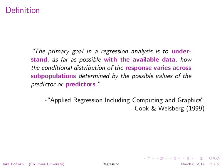
4. Definition “The primary goal in a regression analysis is to under- stand, as far as possible with the available data, how the conditional distribution of the response varies across subpopulations determined by the possible values of the predictor or predictors.” -“Applied Regression Including Computing and Graphics” Cook & Weisberg (1999) Jake Hofman (Columbia University) Regression March 8, 2019 2 / 6
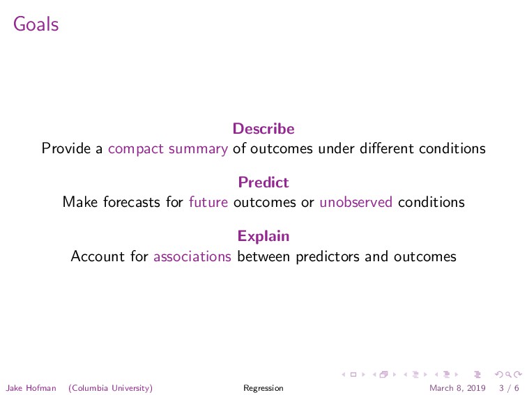
5. Goals Describe Provide a compact summary of outcomes under different conditions Predict Make forecasts for future outcomes or unobserved conditions Explain Account for associations between predictors and outcomes Jake Hofman (Columbia University) Regression March 8, 2019 3 / 6
6. Goals Describe Provide a compact summary of outcomes under different conditions Never “false”, but may be wasteful or misleading Predict Make forecasts for future outcomes or unobserved conditions Varying degrees of success, often room for improvement Explain Account for associations between predictors and outcomes Difficult to establish causality in observational studies See “Regression Analysis: A Constructive Critique”, Berk (2004) Jake Hofman (Columbia University) Regression March 8, 2019 3 / 6
7. Goals Models should be flexible enough to describe observed phenomena but simple enough to generalize to future observations Jake Hofman (Columbia University) Regression March 8, 2019 4 / 6
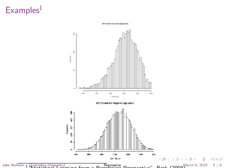
8. Examples1 1.2 Setting the Regression Context 3 Should one be especially interested in a comparison of the means, one could proceed descriptively with a conventional least squares regression analysis as a special case. That is, for each observation i, one could let ˆ yi = β0 + β1 xi , (1.1) where the response variable yi is each applicant’s SAT score, xi is an indicator variable coded “1” if the applicant is Asian and “0” if the applicant is Hispanic, β0 is the mean SAT score for Hispanic applicants, β1 is how much larger (or smaller) the mean SAT score for Asian applicants happens to be, and i is an index running from 1 to the number of Hispanic and Asian applicants, N. Fig. 1.2. Distribution of SAT scores for Asian applicants. SAT Scores for Asian Applicants SAT Score Frequency 600 800 1000 1200 1400 1600 0 50 100 150 to equate regression analysis with causal modeling. This is too narrow and even misleading. Causal modeling is actually an interpretive framework that is imposed on the results of a regression analysis. An alternative knee-jerk response may be to equate regression analysis with the general linear model. At most, the general linear model can be seen as a special case of regression analysis. Statisticians commonly define regression so that the goal is to understand “as far as possible with the available data how the conditional distribution of some response y varies across subpopulations determined by the possible values of the predictor or predictors” (Cook and Weisberg, 1999: 27). That is, interest centers on the distribution of the response variable Y conditioning on one or more predictors X. This definition includes a wide variety of elementary procedures easily implemented in R. (See, for example, Maindonald and Braun, 2007: Chapter 2.) For example, consider Figures 1.1 and 1.2. The first shows the distribution of SAT scores for recent applicants to a major university, who self-identify as “Hispanic.” The second shows the distribution of SAT scores for recent applicants to that same university, who self-identify as “Asian.” 1 Jake Hofman (Columbia University) Regression March 8, 2019 5 / 6
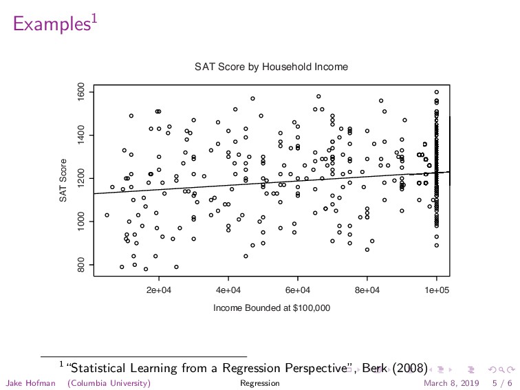
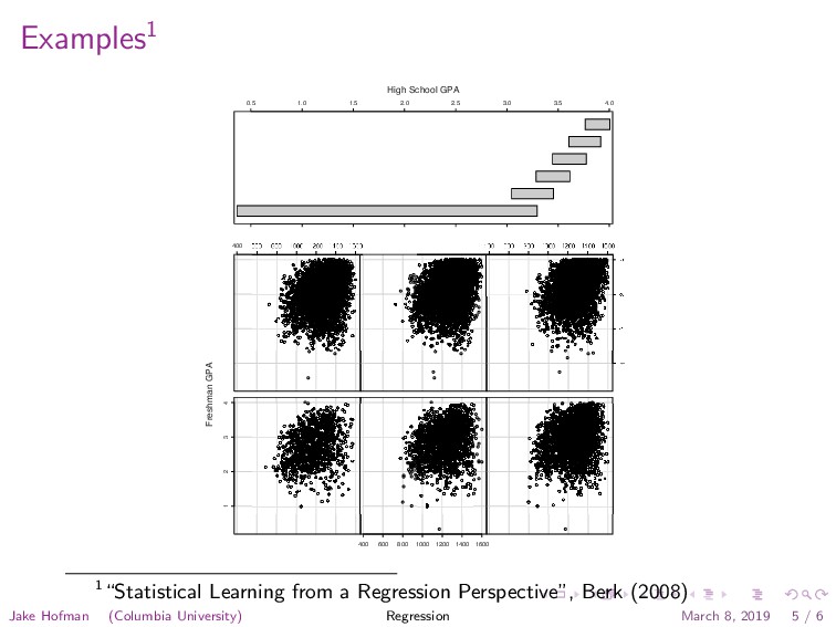
9. Examples1 aph more legible. 2e+04 4e+04 6e+04 8e+04 1e+05 800 1000 1200 1400 1600 SAT Score by Household Income Income Bounded at $100,000 SAT Score Fig. 1.4. SAT scores by family income. 1“Statistical Learning from a Regression Perspective”, Berk (2008) Jake Hofman (Columbia University) Regression March 8, 2019 5 / 6
10. Examples1 6 1 Regression Framework 1 2 3 4 400 600 800 1000 1200 1400 1600 400 600 800 1000 1200 1400 1600 400 600 800 1000 1200 1400 1600 1 2 3 4 Freshman GPA 0.5 1.0 1.5 2.0 2.5 3.0 3.5 4.0 High School GPA Fig. 1.5. Freshman GPA on SAT holding high school GPA constant. 1“Statistical Learning from a Regression Perspective”, Berk (2008) Jake Hofman (Columbia University) Regression March 8, 2019 5 / 6
11. Framework • Specify the outcome and predictors, along with the form of the model relating them • Define a loss function that quantifies how close a model’s predictions are to observed outcomes • Develop an algorithm to fit the model to the observations by minimizing this loss • Assess model performance and interpret results. Jake Hofman (Columbia University) Regression March 8, 2019 6 / 6