Upgrade to Pro — share decks privately, control downloads, hide ads and more …

Modeling Social Data, Lecture 2: Introduction to Counting

Jake Hofman
February 01, 2019

Modeling Social Data, Lecture 2: Introduction to Counting

Jake Hofman

February 01, 2019
Tweet

More Decks by Jake Hofman

Other Decks in Education

Transcript

  1. Introduction to Counting
    APAM E4990
    Modeling Social Data
    Jake Hofman
    Columbia University
    February 1, 2019
    Jake Hofman (Columbia University) Intro to Counting February 1, 2019 1 / 30

    View Slide

  2. Why counting?
    Jake Hofman (Columbia University) Intro to Counting February 1, 2019 2 / 30

    View Slide

  3. Why counting?
    http://bit.ly/august2016poll
    p( y
    support
    | x
    age
    )
    Jake Hofman (Columbia University) Intro to Counting February 1, 2019 3 / 30

    View Slide

  4. Why counting?
    http://bit.ly/ageracepoll2016
    p( y
    support
    | x1, x2
    age, race
    )
    Jake Hofman (Columbia University) Intro to Counting February 1, 2019 3 / 30

    View Slide

  5. Why counting?
    ?
    p( y
    support
    | x1, x2, x3, . . .
    age, sex, race, party
    )
    Jake Hofman (Columbia University) Intro to Counting February 1, 2019 3 / 30

    View Slide

  6. Why counting?
    How many responses do we need to estimate p(y) with a 5%
    margin of error?
    Jake Hofman (Columbia University) Intro to Counting February 1, 2019 4 / 30

    View Slide

  7. Why counting?
    How many responses do we need to estimate p(y) with a 5%
    margin of error?
    What if we want to split this up by age, sex, race, and party?
    Assume ≈ 100 age, 2 sex, 5 race, 3 party
    Jake Hofman (Columbia University) Intro to Counting February 1, 2019 4 / 30

    View Slide

  8. Why counting?
    Problem:
    Traditionally difficult to obtain reliable estimates due to small
    sample sizes or sparsity
    (e.g., ∼ 100 age × 2 sex × 5 race × 3 party = 3,000 groups,
    but typical surveys collect ∼ 1,000s of responses)
    Jake Hofman (Columbia University) Intro to Counting February 1, 2019 5 / 30

    View Slide

  9. Why counting?
    Potential solution:
    Sacrifice granularity for precision, by binning observations into
    larger, but fewer, groups
    (e.g., bin age into a few groups: 18-29, 30-49, 50-64, 65+)
    Jake Hofman (Columbia University) Intro to Counting February 1, 2019 5 / 30

    View Slide

  10. Why counting?
    Potential solution:
    Develop more sophisticated methods that generalize well from
    small samples
    (e.g., fit a model: support ∼ β0 + β1age + β2age2 + . . .)
    Jake Hofman (Columbia University) Intro to Counting February 1, 2019 5 / 30

    View Slide

  11. Why counting?
    (Partial) solution:
    Obtain larger samples through other means, so we can just count
    and divide to make estimates via relative frequencies
    (e.g., with ∼ 1M responses, we have 100s per group and can
    estimate support within a few percentage points)
    Jake Hofman (Columbia University) Intro to Counting February 1, 2019 6 / 30

    View Slide

  12. Why counting?
    International Journal of Forecasting 31 (2015) 980–991
    Contents 
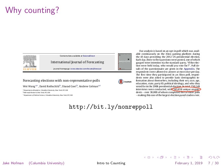
lists available at ScienceDirect
    International Journal of Forecasting
    journal homepage: www.elsevier.com/locate/ijforecast
    Forecasting elections with non-representative polls
    Wei Wanga,⇤
    , David Rothschildb, Sharad Goelb, Andrew Gelmana,c
    a Department of Statistics, Columbia University, New York, NY, USA
    b Microsoft Research, New York, NY, USA
    c Department of Political Science, Columbia University, New York, NY, USA
    a r t i c l e i n f o
    Keywords:
    Non-representative polling
    Multilevel regression and poststratification
    Election forecasting
    a b s t r a c t
    Election forecasts have traditionally been based on representative polls, in which randomly
    sampled individuals are asked who they intend to vote for. While representative polling has
    historically proven to be quite effective, it comes at considerable costs of time and money.
    Moreover, as response rates have declined over the past several decades, the statistical
    benefits of representative sampling have diminished. In this paper, we show that, with
    proper statistical adjustment, non-representative polls can be used to generate accurate
    election forecasts, and that this can often be achieved faster and at a lesser expense than
    traditional survey methods. We demonstrate this approach by creating forecasts from a
    novel and highly non-representative survey dataset: a series of daily voter intention polls
    for the 2012 presidential election conducted on the Xbox gaming platform. After adjusting
    the Xbox responses via multilevel regression and poststratification, we obtain estimates
    which are in line with the forecasts from leading poll analysts, which were based on
    aggregating hundreds of traditional polls conducted during the election cycle. We conclude
    by arguing that non-representative polling shows promise not only for election forecasting,
    but also for measuring public opinion on a broad range of social, economic and cultural
    issues.
    © 2014 International Institute of Forecasters. Published by Elsevier B.V. All rights reserved.
    1. Introduction
    At the heart of modern opinion polling is representative
    sampling, built around the idea that every individual in a
    The wide-scale adoption of representative polling can
    be traced largely back to a pivotal polling mishap in
    the 1936 US presidential election campaign. During
    that campaign, the popular magazine Literary Digest
    W. Wang et al. / International Journal of Forecasting 31 (2015) 980–991 981
    pollsters, including George Gallup, Archibald Crossley, and
    Elmo Roper, used considerably smaller but representative
    samples, and predicted the election outcome with a
    reasonable level of accuracy (Gosnell, 1937). Accordingly,
    non-representative or ‘‘convenience sampling’’ rapidly fell
    out of favor with polling experts.
    So, why do we revisit this seemingly long-settled
    case? Two recent trends spur our investigation. First, ran-
    dom digit dialing (RDD), the standard method in modern
    representative polling, has suffered increasingly high
    non-response rates, due both to the general public’s grow-
    ing reluctance to answer phone surveys, and to expand-
    ing technical means of screening unsolicited calls (Keeter,
    Kennedy, Dimock, Best, & Craighill, 2006). By one mea-
    sure, RDD response rates have decreased from 36% in 1997
    to 9% in 2012 (Kohut, Keeter, Doherty, Dimock, & Chris-
    tian, 2012), and other studies confirm this trend (Holbrook,
    Krosnick, & Pfent, 2007; Steeh, Kirgis, Cannon, & DeWitt,
    2001; Tourangeau & Plewes, 2013). Assuming that the ini-
    tial pool of targets is representative, such low response
    rates mean that those who ultimately answer the phone
    and elect to respond might not be. Even if the selection is-
    sues are not yet a serious problem for accuracy, as some
    have argued (Holbrook et al., 2007), the downward trend
    in response rates suggests an increasing need for post-
    sampling adjustments; indeed, the adjustment methods
    we present here should work just as well for surveys ob-
    tained by probability sampling as for convenience samples.
    The second trend driving our research is the fact that, with
    recent technological innovations, it is increasingly conve-
    nient and cost-effective to collect large numbers of highly
    non-representative samples via online surveys. The data
    that took the Literary Digest editors several months to col-
    lect in 1936 can now take only a few days, and, for some
    surveys, can cost just pennies per response. However, the
    challenge is to extract a meaningful signal from these un-
    conventional samples.
    In this paper, we show that, with proper statistical ad-
    justments, non-representative polls are able to yield ac-
    curate presidential election forecasts, on par with those
    based on traditional representative polls. We proceed as
    follows. Section 2 describes the election survey that we
    conducted on the Xbox gaming platform during the 45
    days leading up to the 2012 US presidential race. Our Xbox
    sample is highly biased in two key demographic dimen-
    how to transform voter intent into projections of vote
    share and electoral votes. We conclude in Section 5 by
    discussing the potential for non-representative polling in
    other domains.
    2. Xbox data
    Our analysis is based on an opt-in poll which was avail-
    able continuously on the Xbox gaming platform during
    the 45 days preceding the 2012 US presidential election.
    Each day, three to five questions were posted, one of which
    gauged voter intention via the standard query, ‘‘If the elec-
    tion were held today, who would you vote for?’’. Full de-
    tails of the questionnaire are given in the Appendix. The
    respondents were allowed to answer at most once per day.
    The first time they participated in an Xbox poll, respon-
    dents were also asked to provide basic demographic in-
    formation about themselves, including their sex, race, age,
    education, state, party ID, political ideology, and who they
    voted for in the 2008 presidential election. In total, 750,148
    interviews were conducted, with 345,858 unique respon-
    dents – over 30,000 of whom completed five or more polls
    – making this one of the largest election panel studies ever.
    Despite the large sample size, the pool of Xbox respon-
    dents is far from being representative of the voting pop-
    ulation. Fig. 1 compares the demographic composition of
    the Xbox participants to that of the general electorate, as
    estimated via the 2012 national exit poll.1 The most strik-
    ing differences are for age and sex. As one might expect,
    young men dominate the Xbox population: 18- to 29-year-
    olds comprise 65% of the Xbox dataset, compared to 19%
    in the exit poll; and men make up 93% of the Xbox sam-
    ple but only 47% of the electorate. Political scientists have
    long observed that both age and sex are strongly correlated
    with voting preferences (Kaufmann & Petrocik, 1999), and
    indeed these discrepancies are apparent in the unadjusted
    time series of Xbox voter intent shown in Fig. 2. In contrast
    to estimates based on traditional, representative polls (in-
    dicated by the dotted blue line in Fig. 2), the uncorrected
    Xbox sample suggests a landslide victory for Mitt Romney,
    reminiscent of the infamous Literary Digest error.
    3. Estimating voter intent with multilevel regression
    and poststratification
    3.1. Multilevel regression and poststratification
    http://bit.ly/nonreppoll
    Jake Hofman (Columbia University) Intro to Counting February 1, 2019 7 / 30
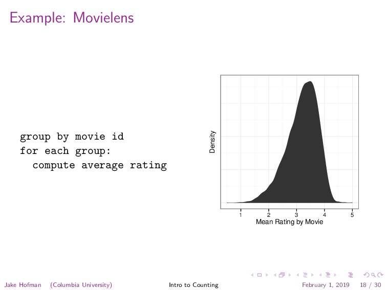
    View Slide

  13. Why counting?
    The good:
    Shift away from sophisticated statistical methods on small samples
    to simpler methods on large samples
    Jake Hofman (Columbia University) Intro to Counting February 1, 2019 8 / 30

    View Slide

  14. Why counting?
    The bad:
    Even simple methods (e.g., counting) are computationally
    challenging at large scales
    (1M is easy, 1B a bit less so, 1T gets interesting)
    Jake Hofman (Columbia University) Intro to Counting February 1, 2019 8 / 30

    View Slide

  15. Why counting?
    Claim:
    Solving the counting problem at scale enables you to investigate
    many interesting questions in the social sciences
    Jake Hofman (Columbia University) Intro to Counting February 1, 2019 8 / 30

    View Slide

  16. Learning to count
    We’ll focus on counting at small/medium scales on a single
    machine
    Jake Hofman (Columbia University) Intro to Counting February 1, 2019 9 / 30

    View Slide

  17. Learning to count
    We’ll focus on counting at small/medium scales on a single
    machine
    But the same ideas extend to counting at large scales on many
    machines
    (Hadoop, Spark, etc.)
    Jake Hofman (Columbia University) Intro to Counting February 1, 2019 9 / 30

    View Slide

  18. Counting, the easy way
    Split / Apply / Combine1
    • Load dataset into memory
    • Split: Arrange observations into groups of interest
    • Apply: Compute distributions and statistics within each group
    • Combine: Collect results across groups
    1http://bit.ly/splitapplycombine
    Jake Hofman (Columbia University) Intro to Counting February 1, 2019 10 / 30

    View Slide

  19. Examples
    How much time and space do we need to compute per-group
    averages?
    Jake Hofman (Columbia University) Intro to Counting February 1, 2019 11 / 30

    View Slide

  20. Examples
    How much time and space do we need to compute per-group
    averages?
    What about per-group variances?
    Jake Hofman (Columbia University) Intro to Counting February 1, 2019 11 / 30

    View Slide

  21. The generic group-by operation
    Split / Apply / Combine
    for each observation as (group, value):
    place value in bucket for corresponding group
    for each group:
    apply a function over values in bucket
    output group and result
    Jake Hofman (Columbia University) Intro to Counting February 1, 2019 12 / 30

    View Slide

  22. The generic group-by operation
    Split / Apply / Combine
    for each observation as (group, value):
    place value in bucket for corresponding group
    for each group:
    apply a function over values in bucket
    output group and result
    Useful for computing arbitrary within-group statistics when we
    have required memory
    (e.g., conditional distribution, median, etc.)
    Jake Hofman (Columbia University) Intro to Counting February 1, 2019 12 / 30

    View Slide

  23. Why counting?
    Jake Hofman (Columbia University) Intro to Counting February 1, 2019 13 / 30

    View Slide

  24. Example: Anatomy of the long tail
    Dataset Users Items Rating levels Observations
    Movielens 100K 10K 10 10M
    Netflix 500K 20K 5 100M
    Jake Hofman (Columbia University) Intro to Counting February 1, 2019 14 / 30

    View Slide

  25. Example: Anatomy of the long tail
    Dataset Users Items Rating levels Observations
    Movielens 100K 10K 10 10M
    Netflix 500K 20K 5 100M
    Jake Hofman (Columbia University) Intro to Counting February 1, 2019 14 / 30

    View Slide

  26. Example: Movielens
    How many ratings are there at each star level?
    0
    1,000,000
    2,000,000
    3,000,000
    1 2 3 4 5
    Rating
    Number of ratings
    Jake Hofman (Columbia University) Intro to Counting February 1, 2019 15 / 30

    View Slide

  27. Example: Movielens
    0
    1,000,000
    2,000,000
    3,000,000
    1 2 3 4 5
    Rating
    Number of ratings
    group by rating value
    for each group:
    count # ratings
    Jake Hofman (Columbia University) Intro to Counting February 1, 2019 16 / 30

    View Slide

  28. Example: Movielens
    What is the distribution of average ratings by movie?
    1 2 3 4 5
    Mean Rating by Movie
    Density
    Jake Hofman (Columbia University) Intro to Counting February 1, 2019 17 / 30

    View Slide

  29. Example: Movielens
    group by movie id
    for each group:
    compute average rating
    1 2 3 4 5
    Mean Rating by Movie
    Density
    Jake Hofman (Columbia University) Intro to Counting February 1, 2019 18 / 30

    View Slide

  30. Example: Movielens
    What fraction of ratings are given to the most popular movies?
    0%
    25%
    50%
    75%
    100%
    0 3,000 6,000 9,000
    Movie Rank
    CDF
    Jake Hofman (Columbia University) Intro to Counting February 1, 2019 19 / 30

    View Slide

  31. Example: Movielens
    0%
    25%
    50%
    75%
    100%
    0 3,000 6,000 9,000
    Movie Rank
    CDF
    group by movie id
    for each group:
    count # ratings
    sort by group size
    cumulatively sum group sizes
    Jake Hofman (Columbia University) Intro to Counting February 1, 2019 20 / 30

    View Slide

  32. Example: Movielens
    What is the median rank of each user’s rated movies?
    0
    2,000
    4,000
    6,000
    8,000
    100 10,000
    User eccentricity
    Number of users
    Jake Hofman (Columbia University) Intro to Counting February 1, 2019 21 / 30

    View Slide

  33. Example: Movielens
    join movie ranks to ratings
    group by user id
    for each group:
    compute median movie rank
    0
    2,000
    4,000
    6,000
    8,000
    100 10,000
    User eccentricity
    Number of users
    Jake Hofman (Columbia University) Intro to Counting February 1, 2019 22 / 30

    View Slide

  34. Example: Anatomy of the long tail
    Dataset Users Items Rating levels Observations
    Movielens 100K 10K 10 10M
    Netflix 500K 20K 5 100M
    What do we do when the full dataset exceeds available memory?
    Jake Hofman (Columbia University) Intro to Counting February 1, 2019 23 / 30

    View Slide

  35. Example: Anatomy of the long tail
    Dataset Users Items Rating levels Observations
    Movielens 100K 10K 10 10M
    Netflix 500K 20K 5 100M
    What do we do when the full dataset exceeds available memory?
    Sampling?
    Unreliable estimates for rare groups
    Jake Hofman (Columbia University) Intro to Counting February 1, 2019 23 / 30

    View Slide

  36. Example: Anatomy of the long tail
    Dataset Users Items Rating levels Observations
    Movielens 100K 10K 10 10M
    Netflix 500K 20K 5 100M
    What do we do when the full dataset exceeds available memory?
    Random access from disk?
    1000x more storage, but 1000x slower2
    2Numbers every programmer should know
    Jake Hofman (Columbia University) Intro to Counting February 1, 2019 23 / 30

    View Slide

  37. Example: Anatomy of the long tail
    Dataset Users Items Rating levels Observations
    Movielens 100K 10K 10 10M
    Netflix 500K 20K 5 100M
    What do we do when the full dataset exceeds available memory?
    Streaming
    Read data one observation at a time, storing only needed state
    Jake Hofman (Columbia University) Intro to Counting February 1, 2019 23 / 30

    View Slide

  38. The combinable group-by operation
    Streaming
    for each observation as (group, value):
    if new group:
    initialize result
    update result for corresponding group as function of
    existing result and current value
    for each group:
    output group and result
    Jake Hofman (Columbia University) Intro to Counting February 1, 2019 24 / 30

    View Slide

  39. The combinable group-by operation
    Streaming
    for each observation as (group, value):
    if new group:
    initialize result
    update result for corresponding group as function of
    existing result and current value
    for each group:
    output group and result
    Useful for computing a subset of within-group statistics with a
    limited memory footprint
    (e.g., min, mean, max, variance, etc.)
    Jake Hofman (Columbia University) Intro to Counting February 1, 2019 24 / 30

    View Slide

  40. Example: Movielens
    0
    1,000,000
    2,000,000
    3,000,000
    1 2 3 4 5
    Rating
    Number of ratings
    for each rating:
    counts[movie id]++
    Jake Hofman (Columbia University) Intro to Counting February 1, 2019 25 / 30

    View Slide

  41. Example: Movielens
    for each rating:
    totals[movie id] += rating
    counts[movie id]++
    for each group:
    totals[movie id] /
    counts[movie id]
    1 2 3 4 5
    Mean Rating by Movie
    Density
    Jake Hofman (Columbia University) Intro to Counting February 1, 2019 26 / 30

    View Slide

  42. Yet another group-by operation
    Per-group histograms
    for each observation as (group, value):
    histogram[group][value]++
    for each group:
    compute result as a function of histogram
    output group and result
    Jake Hofman (Columbia University) Intro to Counting February 1, 2019 27 / 30

    View Slide

  43. Yet another group-by operation
    Per-group histograms
    for each observation as (group, value):
    histogram[group][value]++
    for each group:
    compute result as a function of histogram
    output group and result
    We can recover arbitrary statistics if we can afford to store counts
    of all distinct values within in each group
    Jake Hofman (Columbia University) Intro to Counting February 1, 2019 27 / 30

    View Slide

  44. The group-by operation
    For arbitrary input data:
    Memory Scenario Distributions Statistics
    N Small dataset Yes General
    V*G Small distributions Yes General
    G Small # groups No Combinable
    V Small # outcomes No No
    1 Large # both No No
    N = total number of observations
    G = number of distinct groups
    V = largest number of distinct values within group
    Jake Hofman (Columbia University) Intro to Counting February 1, 2019 28 / 30

    View Slide

  45. Examples (w/ 8GB RAM)
    Median rating by movie for Netflix
    N ∼ 100M ratings
    G ∼ 20K movies
    V ∼ 10 half-star values
    V *G ∼ 200K, store per-group histograms for arbitrary statistics
    (scales to arbitrary N, if you’re patient)
    Jake Hofman (Columbia University) Intro to Counting February 1, 2019 29 / 30

    View Slide

  46. Examples (w/ 8GB RAM)
    Median rating by video for YouTube
    N ∼ 10B ratings
    G ∼ 1B videos
    V ∼ 10 half-star values
    V *G ∼ 10B, fails because per-group histograms are too large to
    store in memory
    G ∼ 1B, but no (exact) calculation for streaming median
    Jake Hofman (Columbia University) Intro to Counting February 1, 2019 29 / 30

    View Slide

  47. Examples (w/ 8GB RAM)
    Mean rating by video for YouTube
    N ∼ 10B ratings
    G ∼ 1B videos
    V ∼ 10 half-star values
    G ∼ 1B, use streaming to compute combinable statistics
    Jake Hofman (Columbia University) Intro to Counting February 1, 2019 29 / 30

    View Slide

  48. The group-by operation
    For pre-grouped input data:
    Memory Scenario Distributions Statistics
    N Small dataset Yes General
    V*G Small distributions Yes General
    G Small # groups No Combinable
    V Small # outcomes Yes General
    1 Large # both No Combinable
    N = total number of observations
    G = number of distinct groups
    V = largest number of distinct values within group
    Jake Hofman (Columbia University) Intro to Counting February 1, 2019 30 / 30

    View Slide