Modeling Social Data, Lecture 9: Classification

Transcript

1. Classification: Naive Bayes APAM E4990 Modeling Social Data Jake Hofman Columbia University March 29, 2019 Jake Hofman (Columbia University) Classification: Naive Bayes March 29, 2019 1 / 16
2. Learning by example Jake Hofman (Columbia University) Classification: Naive Bayes March 29, 2019 2 / 16
3. Learning by example • How did you solve this problem? • Can you make this process explicit (e.g. write code to do so)? Jake Hofman (Columbia University) Classification: Naive Bayes March 29, 2019 2 / 16
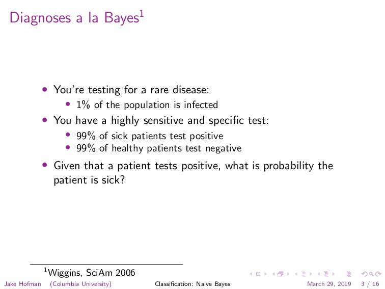
4. Diagnoses a la Bayes1 • You’re testing for a rare disease: • 1% of the population is infected • You have a highly sensitive and specific test: • 99% of sick patients test positive • 99% of healthy patients test negative • Given that a patient tests positive, what is probability the patient is sick? 1Wiggins, SciAm 2006 Jake Hofman (Columbia University) Classification: Naive Bayes March 29, 2019 3 / 16
5. Diagnoses a la Bayes Population 10,000 ppl 1% Sick 100 ppl 99% Test + 99 ppl 1% Test - 1 per 99% Healthy 9900 ppl 1% Test + 99 ppl 99% Test - 9801 ppl Jake Hofman (Columbia University) Classification: Naive Bayes March 29, 2019 4 / 16
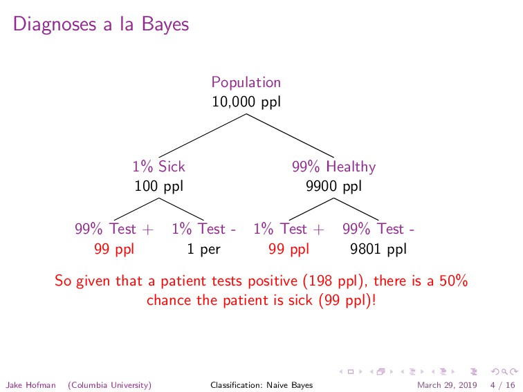
6. Diagnoses a la Bayes Population 10,000 ppl 1% Sick 100 ppl 99% Test + 99 ppl 1% Test - 1 per 99% Healthy 9900 ppl 1% Test + 99 ppl 99% Test - 9801 ppl So given that a patient tests positive (198 ppl), there is a 50% chance the patient is sick (99 ppl)! Jake Hofman (Columbia University) Classification: Naive Bayes March 29, 2019 4 / 16
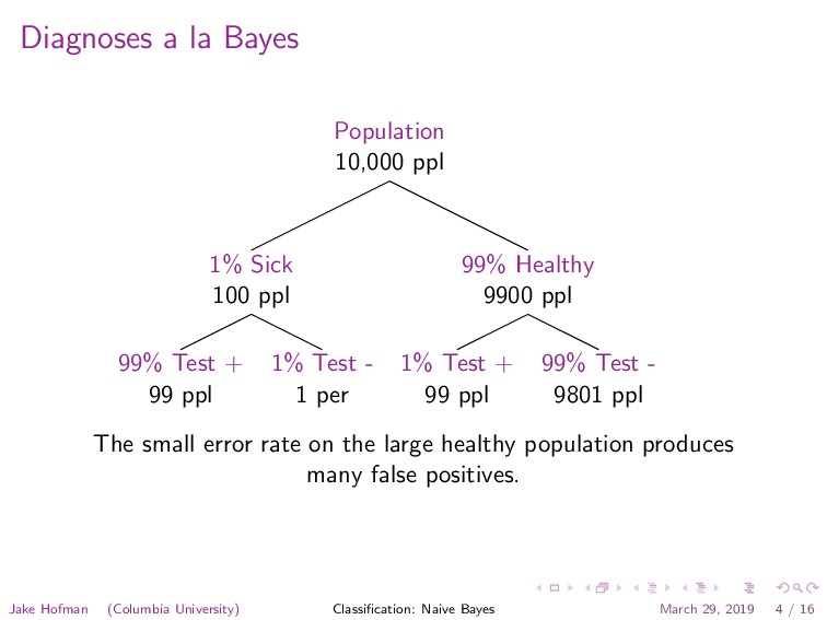
7. Diagnoses a la Bayes Population 10,000 ppl 1% Sick 100 ppl 99% Test + 99 ppl 1% Test - 1 per 99% Healthy 9900 ppl 1% Test + 99 ppl 99% Test - 9801 ppl The small error rate on the large healthy population produces many false positives. Jake Hofman (Columbia University) Classification: Naive Bayes March 29, 2019 4 / 16
8. Natural frequencies a la Gigerenzer2 2http://bit.ly/ggbbc Jake Hofman (Columbia University) Classification: Naive Bayes March 29, 2019 5 / 16
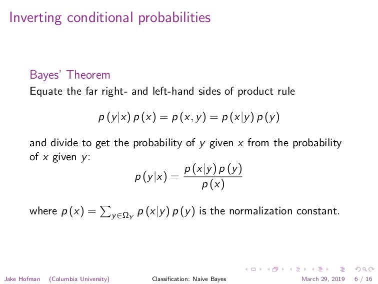
9. Inverting conditional probabilities Bayes’ Theorem Equate the far right- and left-hand sides of product rule p (y|x) p (x) = p (x, y) = p (x|y) p (y) and divide to get the probability of y given x from the probability of x given y: p (y|x) = p (x|y) p (y) p (x) where p (x) = y∈ΩY p (x|y) p (y) is the normalization constant. Jake Hofman (Columbia University) Classification: Naive Bayes March 29, 2019 6 / 16
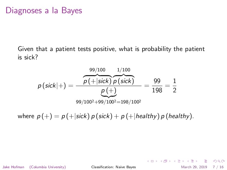
10. Diagnoses a la Bayes Given that a patient tests positive, what is probability the patient is sick? p (sick|+) = 99/100 p (+|sick) 1/100 p (sick) p (+) 99/1002+99/1002=198/1002 = 99 198 = 1 2 where p (+) = p (+|sick) p (sick) + p (+|healthy) p (healthy). Jake Hofman (Columbia University) Classification: Naive Bayes March 29, 2019 7 / 16
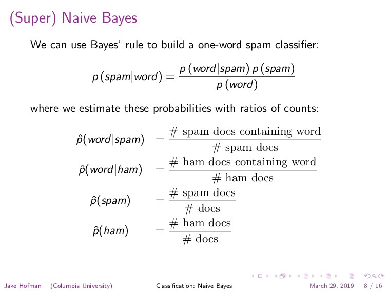
11. (Super) Naive Bayes We can use Bayes’ rule to build a one-word spam classifier: p (spam|word) = p (word|spam) p (spam) p (word) where we estimate these probabilities with ratios of counts: ˆ p(word|spam) = # spam docs containing word # spam docs ˆ p(word|ham) = # ham docs containing word # ham docs ˆ p(spam) = # spam docs # docs ˆ p(ham) = # ham docs # docs Jake Hofman (Columbia University) Classification: Naive Bayes March 29, 2019 8 / 16
12. (Super) Naive Bayes $ ./enron_naive_bayes.sh meeting 1500 spam examples 3672 ham examples 16 spam examples containing meeting 153 ham examples containing meeting estimated P(spam) = .2900 estimated P(ham) = .7100 estimated P(meeting|spam) = .0106 estimated P(meeting|ham) = .0416 P(spam|meeting) = .0923 Jake Hofman (Columbia University) Classification: Naive Bayes March 29, 2019 9 / 16
13. (Super) Naive Bayes $ ./enron_naive_bayes.sh money 1500 spam examples 3672 ham examples 194 spam examples containing money 50 ham examples containing money estimated P(spam) = .2900 estimated P(ham) = .7100 estimated P(money|spam) = .1293 estimated P(money|ham) = .0136 P(spam|money) = .7957 Jake Hofman (Columbia University) Classification: Naive Bayes March 29, 2019 10 / 16
14. (Super) Naive Bayes $ ./enron_naive_bayes.sh enron 1500 spam examples 3672 ham examples 0 spam examples containing enron 1478 ham examples containing enron estimated P(spam) = .2900 estimated P(ham) = .7100 estimated P(enron|spam) = 0 estimated P(enron|ham) = .4025 P(spam|enron) = 0 Jake Hofman (Columbia University) Classification: Naive Bayes March 29, 2019 11 / 16
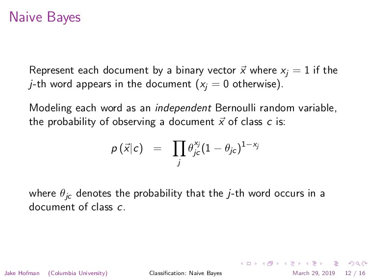
15. Naive Bayes Represent each document by a binary vector x where xj = 1 if the j-th word appears in the document (xj = 0 otherwise). Modeling each word as an independent Bernoulli random variable, the probability of observing a document x of class c is: p (x|c) = j θxj jc (1 − θjc)1−xj where θjc denotes the probability that the j-th word occurs in a document of class c. Jake Hofman (Columbia University) Classification: Naive Bayes March 29, 2019 12 / 16
16. Naive Bayes Using this likelihood in Bayes’ rule and taking a logarithm, we have: log p (c|x) = log p (x|c) p (c) p (x) = j xj log θjc 1 − θjc + j log(1 − θjc) + log θc p (x) where θc is the probability of observing a document of class c. Jake Hofman (Columbia University) Classification: Naive Bayes March 29, 2019 13 / 16
17. Naive Bayes We can eliminate p (x) by calculating the log-odds: log p (1|x) p (0|x) = j xj log θj1(1 − θj0) θj0(1 − θj1) wj + j log 1 − θj1 1 − θj0 + log θ1 θ0 w0 which gives a linear classifier of the form w · x + w0 Jake Hofman (Columbia University) Classification: Naive Bayes March 29, 2019 14 / 16
18. Naive Bayes We train by counting words and documents within classes to estimate θjc and θc: ˆ θjc = njc nc ˆ θc = nc n and use these to calculate the weights ˆ wj and bias ˆ w0: ˆ wj = log ˆ θj1(1 − ˆ θj0) ˆ θj0(1 − ˆ θj1) ˆ w0 = j log 1 − ˆ θj1 1 − ˆ θj0 + log ˆ θ1 ˆ θ0 . We we predict by simply adding the weights of the words that appear in the document to the bias term. Jake Hofman (Columbia University) Classification: Naive Bayes March 29, 2019 15 / 16
19. Naive Bayes In practice, this works better than one might expect given its simplicity3 3http://www.jstor.org/pss/1403452 Jake Hofman (Columbia University) Classification: Naive Bayes March 29, 2019 16 / 16
20. Naive Bayes Training is computationally cheap and scalable, and the model is easy to update given new observations3 3http://www.springerlink.com/content/wu3g458834583125/ Jake Hofman (Columbia University) Classification: Naive Bayes March 29, 2019 16 / 16
21. Naive Bayes Performance varies with document representations and corresponding likelihood models3 3http://ceas.cc/2006/15.pdf Jake Hofman (Columbia University) Classification: Naive Bayes March 29, 2019 16 / 16
22. Naive Bayes It’s often important to smooth parameter estimates (e.g., by adding pseudocounts) to avoid overfitting ˆ θjc = njc + α nc + α + β Jake Hofman (Columbia University) Classification: Naive Bayes March 29, 2019 16 / 16
23. Measures of success Jake Hofman (Columbia University) Classification: Naive Bayes March 29, 2019 17 / 16
24. Measures of success Accuracy: The fraction of examples correctly classified Jake Hofman (Columbia University) Classification: Naive Bayes March 29, 2019 18 / 16
25. Measures of success Precision: The fraction of predicted spam that’s actually spam Jake Hofman (Columbia University) Classification: Naive Bayes March 29, 2019 18 / 16
26. Measures of success Recall: The fraction of all spam that’s predicted to be spam Jake Hofman (Columbia University) Classification: Naive Bayes March 29, 2019 18 / 16
27. Measures of success False positive rate: The fraction of legitimate email that’s predicted to be spam Jake Hofman (Columbia University) Classification: Naive Bayes March 29, 2019 18 / 16