Tutorial: Understanding and Modelling Defects in Semiconductors (with VASP)

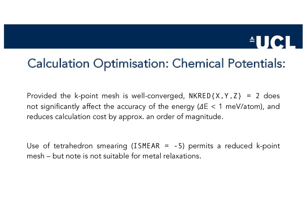
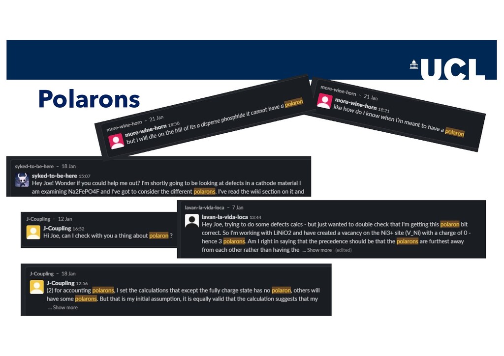
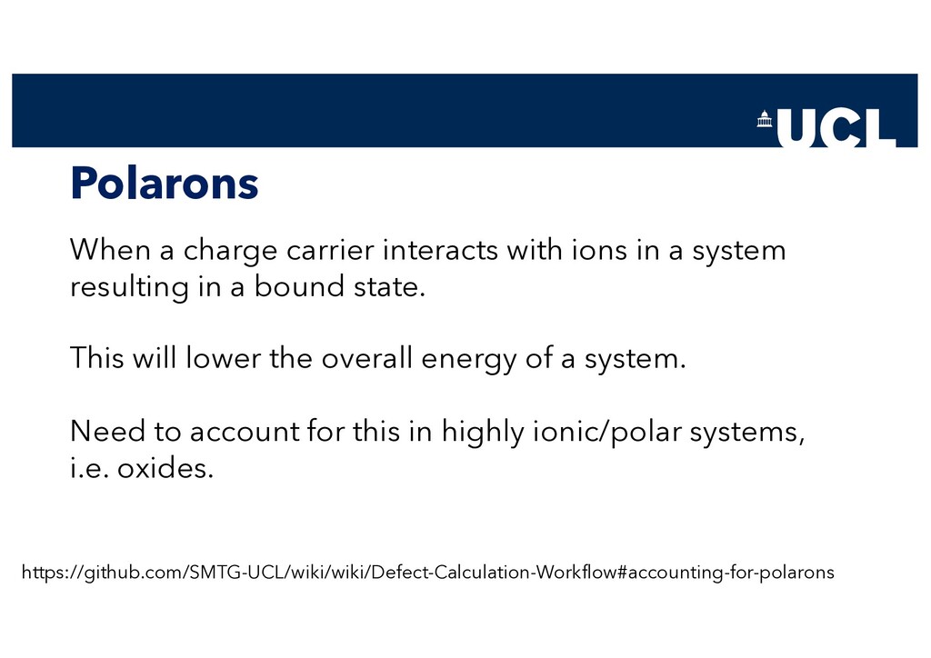
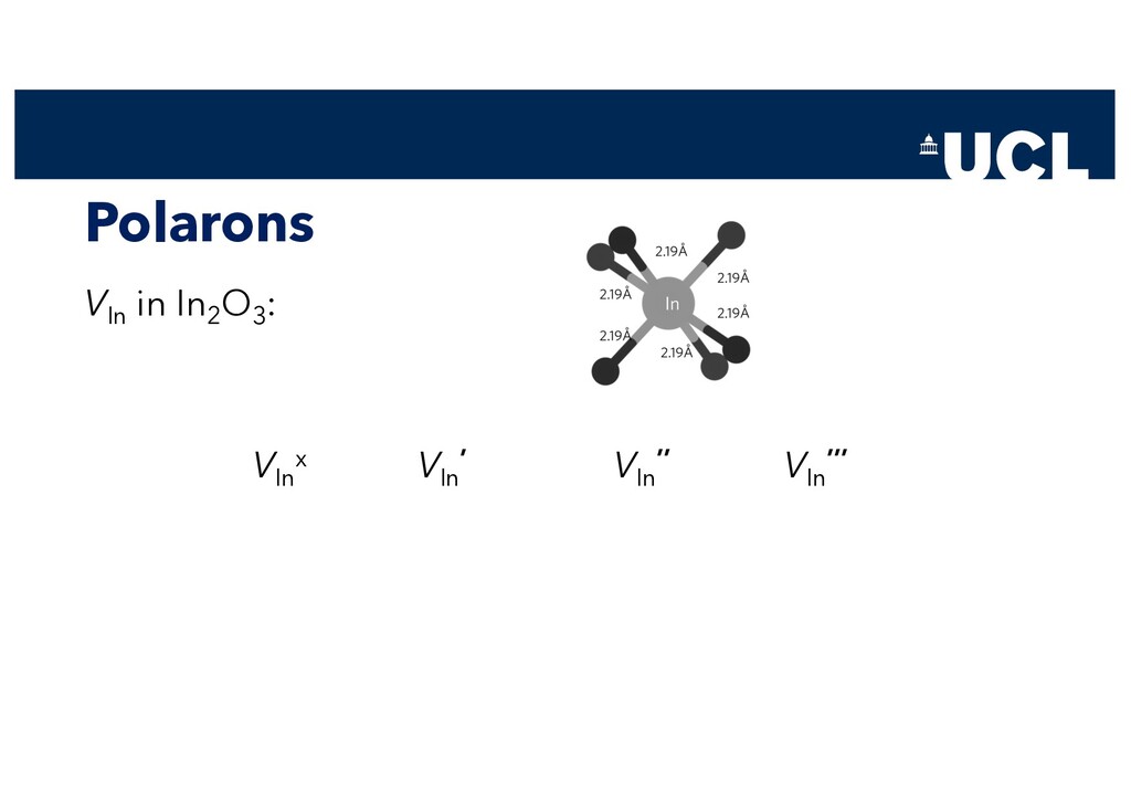
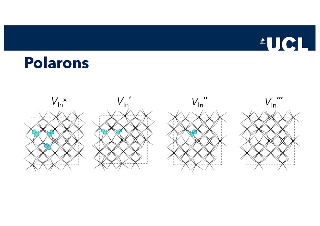
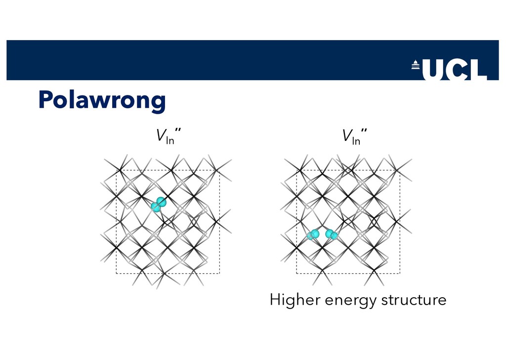
Slides from a tutorial talk at the Scanlon Materials Theory Group, joint with Joe Willis, on understanding and computationally modelling defects in semiconductors.

If you're interested in this work, please check out our open-access review on perovskite-inspired materials and defect tolerance here:
https://iopscience.iop.org/article/10.1088/1361-6528/abcf6d

For other research articles see:
https://bit.ly/3pBMxOG

For other talks on YouTube see:
https://bit.ly/2U5YgLf

Transcript

1. Defects Tutorial I: Fundamentals Seán R. Kavanagh & Joe Willis 21/01/2021
2. Overview This time… § Motivation § Types of defect § Formation energies § Transition level diagrams § Understanding results § Experimental defects Next time… § Calculations § INCAR settings § Dos and don’ts
3. Motivation § Defects control device behaviour
4. Point Defect Classification Intrinsic: Defect arising from imperfect arrangement of the bulk atoms. Always present; concentrations can be controlled just with temperature. Extrinsic: Defect arising from an external impurity. (e.g. doping, intentional or otherwise). Vacancy: Missing atom at lattice site. Interstitial: Atom located at interstitial site (i.e. void in the crystal structure). Substitution: Atom located at the lattice site of a different element. (Often “Antisite” if intrinsic). Complex: Two or more point defects located nearby, with elastic/electronic/magnetic/etc interactions.
5. Kröger–Vink Point Defect Notation X is the species: - Element (Si, Cd…) - Vacancy “V” or “v” S is the lattice site: - Elemental Symbol of original site - “i” for an interstitial site q is the electronic charge of the species relative to the site that it occupies - q = Current Charge – Original Charge Kröger- Vink (Chemistry) Materials Science × 0 ′′ -2 •• +2 Charge Notation:
6. Kröger–Vink Point Defect Notation
7. Defect Formation Energy § Overview Goyal, A. et al, Comp. Mat. Sci., 2017, 130, 1-9
8. Supercells § D = defect § q = charge state § H = host
9. Chemical Potential § Accounting for the change in Gibbs free energy when adding or removing an atom § ni = number of atoms added to (negative) or removed from (positive) the host § µi = chemical potential § i = atomic species … but what is it?
10. Chemical Potential: Definition § Rate of change of free energy of a system with respect to the change in number of atoms in the system, i.e.
11. Chemical Potential: Limits § Thermodynamic stability of host material, e.g. ZnO
12. Chemical Potential: Limits Zn-rich: Zn-poor:
13. Chemical Potential: Limits § For multiple stable competing phases, solve simultaneous equations:
14. Chemical Potential: Limits https://github.com/SMTG-UCL/wiki/wiki/Defects:-Chemical-Potential-Limits § For TiO2 :
15. Chemical Potential: Dopant Limits § For a VTi defect: § The same process can be applied for dopant competing phases, but within chemical potential limits of the host material
16. Chemical Potential: Dopant Limits Species Ti rich Ti poor Nb2 O5 -0.44 -9.24 NbO2 -0.42 -7.46 NbO -0.58 -4.10 µO = -3.52 µO = 0 µ Ti rich Ti poor Ti -2.10 -9.14 O -3.52 0.00 Nb -0.58 -9.24
17. Chemical Potential: Doping Limits § For a substitution, you now must account for the energy needed to remove a host atom and to add a dopant atom § e.g. for a NbTi defect:
18. Defect Formation Energy Goyal A, Gorai P, Peng H, Lany S and Stevanović V 2017 A computational framework for automation of point defect calculations Comput. Mater. Sci. 130 1–9 Fermi level = the thermodynamic work required to add one electron to the system
19. Defect Formation Energy Goyal A, Gorai P, Peng H, Lany S and Stevanović V 2017 A computational framework for automation of point defect calculations Comput. Mater. Sci. 130 1–9 Defect-Defect Interactions:
20. Defect Formation Energy § Overview Goyal, A. et al, Comp. Mat. Sci., 2017, 130, 1-9
21. Transition Level Diagram
22. Fermi Level EF / eV Formation energy / eV 𝑦 = 𝑚𝑥 + 𝑐 Fermi Level EF / eV Formation energy / eV +1 0 -1
23. Transition Level Diagram Fermi Level EF / eV Formation energy / eV +1 0 -1
24. Deep Defect Fermi Level EF / eV Formation energy / eV +1 0 0 3 CBM
25. Deep Defect Huang, Y.-T. et al, Nano., 2021, 32, 132004
26. Shallow Defect Fermi Level EF / eV Formation energy / eV +1 0 0 3 CBM
27. Resonant Defect Fermi Level EF / eV Formation energy / eV +1 0 0 3 CBM
28. Comparing Chemical Potential Limits
29. Thermodynamic Driving Forces of Disorder Thermodynamic equilibrium: ΔF is minimised Gibbs Free Energy ΔF = ΔH – TΔS Configurational entropy S = kB lnW kB. = Boltzmann constant W = Multiplicity (of defect formation) Energy Free Energy Minimum (Thermodynamic Equilibrium) nd Nexp −∆H kB T Image Credits: Prof. Graeme Watson
31. Defect Formation Energy Diagrams Fermi Level Pinning Charge Neutrality: p + ND + = n + NA – EF
32. Defect Formation Energy Diagrams Fermi Level Pinning Charge Neutrality: p + ND + = n + NA – EF
33. Defect Formation Energy Diagrams Fermi Level Pinning Charge Neutrality: p + ND + = n + NA – EF
34. Defect Formation Energy Diagrams Fermi Level Pinning Charge Neutrality: p + ND + = n + NA – EF
35. Defect Properties: Optical Transition Levels Td C3v Configuration Coordinate (Q) 0.0 0.1 0.2 0.3 0.4 0.5 0.6 0.7 Relative Energy (eV) 0.47 eV 0.22 eV 0.36 eV 0.58 eV 2.61 Å 2.59 Å 3.05 Å
36. Optical Transition Levels
37. Defect Formation Energy Diagrams Deep, shallow or resonant?
38. Defect Formation Energy Diagrams Deep Levels -> Efficiency Reduction in Solar Cells
39. Experiment - HAXPES HAXPES Credit: T. J. Featherstone
40. Experiment - DLTS Lang, D. V., Jour. Appl. Phys., 1974, 45, 3023-32
41. Experiment – DLTS Scanlon, D. O. et al, PRL, 2009, 103, 096405
42. Next Time § More complicated chemical potential spaces § How to set up calculations § Finite size corrections in practice § Polarons § Optical transitions
43. Further Reading § Lany, S. and Zunger, A., Phys. Rev. B, 2008, 78, 235104 § Freysoldt, C. et al, Rev. Mod. Phys., 2014, 86, 253 § Williamson, B. A. D. et al, Chem. Mater., 2020, 32, 1964-73 § Swallow, J. E. N. et al, Mater. Horiz., 2020, 7, 236-43 § Wickramaratne, D. et al, Appl. Phys. Lett., 2018, 113, 192106
44. Chemical Potential: Ternary + § The problem clearly gets larger with more competing phases and more complex materials. § Use CPLAP! § Input: https://github.com/jbuckeridge/cplap
45. Chemical Potential: Ternary + § Output:
46. Chemical Potential: Ternary + Ternary: § 2D x-y plot with colour chart as 3rd dimension § 3D x-y-z plot For quaternary: § 3D x-y-z- plot with colour chart as 4th dimension § 2D x-y plots with colour chart as 3rd dimension, keep one chemical potential constant § 2D x-y plots keep two chemical potentials constant
47. Chemical Potentials: Quaternary Example § Overview Xiao, Z. et al, Adv. Func. Mater., 2020, 1909906
48. Defects Tutorial II: Implementation Seán R. Kavanagh & Joe Willis 04/02/2020
49. Overview § Primitive – supercell relationship § Constructing defective supercells § INCAR tags § Calculating defects efficiently § Finite correction schemes in practice § Polarons § CPLAP for complex systems § Summary
50. From primitive to supercell 3 x 3 x 2 $ super –f POSCAR 3 3 2 Initial structure has 4 atoms Final structure has 72 atoms import pymatgen.core.structure make_supercell(scaling_matrix)
51. From primitive to supercell $ kgrid-series POSCAR_prim Length cutoff KSPACING Samples ------------- -------- ------------ 10.419 0.3015 8 8 4 $ kgrid-series POSCAR_super_3_3_2 Length cutoff KSPACING Samples ------------- -------- ------------ 10.419 0.3015 3 3 2 IMPORTANT Remember the relationship between real and reciprocal space Change your k-point grid accordingly
52. Creating Point Defects • Manual • Python 🐍
53. Creating Point Defects: Manual
54. Creating Point Defects: Manual POSCAR: Beware POSCAR elemental ordering!
55. Creating Point Defects: Python
56. Creating Point Defects: Python github.com/kavanase/doped
57. INCAR tags Bread and butter tags: ISIF = 2 ISYM = 0 IBRION = 1 POTIM = 0.2 ISPIN = 2 Play around with as usual if relaxation is getting stuck
58. INCAR tags Trade-off between accuracy and supercell size/number of electrons in system: LREAL = False or LREAL = Auto ROPT = 1E-03 ! For each species in POSCAR Fast! More accurate, may be required for non- convergent relaxations
59. INCAR tags If using AIDE: ICORELEVEL = 0 or 1 LVHAR = .TRUE. 0 prints average electrostatic potential at core 1 prints core state eigenenergies AIDE will calculate potential alignment using either. Be consistent across your project!
60. INCAR tags If using DOPED: LVHAR = .TRUE. or ICORELEVEL = 0 Freysoldt Kumagai More on this from Seán to come…
61. INCAR tags Setting charge states: 1. DOPED – reads POSCAR and POTCAR and assigns charge states based on pymatgen.core module. Can then manually pick/delete charge states provided. 2. Manually for AIDE – use your chemical intuition to consider each defect site and change NELECT and NUPDOWN accordingly.
62. Chemical intuition…
63. INCAR tags VO in In2 O3 : … or just use DOPED! VO x VO • VO •• NUPDOWN sets the difference between the number of electrons in the spin up and spin down channels. NELECT sets total number of electrons. NELECT = 378 NUPDOWN = 0 NELECT = 377 NUPDOWN = 1 NELECT = 376 NUPDOWN = 0
64. Calculation Optimisation: Converge Test! davidbowler.github.io/AtomisticSimulations/blog/dft-scaling DFT Computation Time ∝ N3 Hybrid DFT ∝ N3 – N4 github.com/kavanase/vaspup2.0
65. Calculation Optimisation: Test your System ‘Spot the difference’
66. Calculation Optimisation: Test your System • AlGO • Supercell Size and k- grid combinations • KPAR
67. Calculation Optimisation: Relaxation Pre-Convergence 𝚪-point only vasp_g am • For each inequivale nt defect site and likely magnetic configurat ion. NKRED = 2 vasp_s td • Only the lowest energy vasp_gam - predicted configurat ion, vasp_ std • Continua tion from NKRED run (often only 1 or 2 steps). vasp_ ncl • Spin-orbit single- shot energy calculatio n (possibly with (Can’t use WAVECAR from vasp_gam) (Can’t use WAVECAR from vasp_std)
68. Calculation Optimisation: Relaxation Pre-Convergence 𝚪-point only vasp_gam •For each inequivalent defect site and likely magnetic configuration. NKRED = 2 vasp_std •Only the lowest energy vasp_gam- predicted configuration, unless tiny 𝛥E. vasp_std •Continuation from NKRED run (often only 1 or 2 steps). vasp_ncl •Spin-orbit single-shot energy calculation (possibly with ISMEAR=-5) (Can’t use WAVECAR from vasp_gam) (Can’t use WAVECAR from vasp_std)
69. Post-Processing: Finite-Size Corrections AIDE (Lany-Zunger Correction Scheme) defects.dat: chem_pots.dat -> Chemical Potentials limits.dat -> Chemical Potential Limits diel.dat -> Dielectric Tensor
70. Post-Processing: Finite-Size Corrections doped (FNV, Kumagai & Oba or Lany-Zunger Correction Scheme)
71. Calculation Optimisation: Chemical Potentials: Smearing 5 10 15 20 25 30 k-point Mesh (i x i x i) −60 −50 −40 −30 −20 −10 0 10 Ground-State Energy wrt Converged Value [meV] Energy Convergence wrt k-point Mesh ISMEAR = -5 ISMEAR = 2 ISMEAR = 0 Good k-point convergence particularly important for calculations of metallic phases. (Metallic Bismuth)
72. Calculation Optimisation: Chemical Potentials: Provided the k-point mesh is well-converged, NKRED{X,Y,Z} = 2 does not significantly affect the accuracy of the energy (𝛥E < 1 meV/atom), and reduces calculation cost by approx. an order of magnitude. Use of tetrahedron smearing (ISMEAR = -5) permits a reduced k-point mesh – but note is not suitable for metal relaxations.
73. Polarons
74. Polarons When a charge carrier interacts with ions in a system resulting in a bound state. This will lower the overall energy of a system. Need to account for this in highly ionic/polar systems, i.e. oxides. https://github.com/SMTG-UCL/wiki/wiki/Defect-Calculation-Workflow#accounting-for-polarons
75. Polarons VIn in In2 O3 : VIn x VIn ’ VIn ’’ VIn ’’’
76. Polarons VIn x 3 holes NELECT = 381 MAGMOM sets the initial magnetic moment for each atom NUPDOWN = 1 MAGMOM = 31*0 45*0 2*1 1*-1 NUPDOWN = 3 MAGMOM = 31*0 45*0 3*1 POSCAR In O 31 48
77. Polarons VIn ’ 2 holes NUPDOWN = 2 MAGMOM = 31*0 46*0 2*1 POSCAR In O 31 48 NELECT = 382 NUPDOWN = 0 MAGMOM = 31*0 46*0 1*1 1*-1
78. Polarons VIn ’’ 1 hole NUPDOWN = 1 MAGMOM = 31*0 47*0 1*1 POSCAR In O 31 48 NELECT = 383
79. Polarons VIn ’’’ 0 holes NUPDOWN = 0 MAGMOM = 31*0 48*0 POSCAR In O 31 48 NELECT = 384
80. Polarons VIn x VIn ’ VIn ’’ VIn ’’’
81. Polawrong VIn ’’ VIn ’’ Higher energy structure
82. Polarons Consider the ionicity of your material. Less likely in materials with disperse VBMs. Test all combinations with vasp_gam. Visualise hole charge density using PARCHG file. (Apply reverse logic if expecting localized electrons) https://github.com/SMTG-UCL/wiki/wiki/VASP-Partial-Charges
83. CPLAP Chemical Potential Limits Analysis Program. Calculates values of µ for all elements in complex chemical potential spaces. Example run through with ternary material BaSnO3 .
84. CPLAP 1. Calculate elemental reference energies. 2. Calculate formation energies of all stable competing phases (NOTE energy per formula unit) 3. Run CPLAP.
85. CPLAP Sample input file: 3 !Number of species in host compound. 1 Ba 1 Sn 3 O -11.464243 !Stoichiometry + formation energy. none !Dependent variable. 3 !Number of competing phases. 2 !Number of species in comp. phase. 1 Ba 1 O -5.1386635 !Stoichiometry + formation energy. 2 !Number of species in comp. phase. 1 Sn 1 O -2.539629 !Stoichiometry + formation energy. 2 !Number of species in comp. phase. 1 Sn 2 O -5.2876295 !Stoichiometry + formation energy.
86. CPLAP Sample output file Intersection points in chemical potential space: mu_Ba mu_Sn | mu_O = ----------------------|----------- -1.9759 0.0000 | -3.1628 -5.1387 -6.3256 | 0.0000 -3.5328 0.0000 | -2.6438 -6.1766 -5.2876 | 0.0000 -2.4948 0.0000 | -2.9898 -5.1387 -5.2876 | -0.3460 O-poor O-rich O-rich
87. CPLAP Plotting: • 3D xyz plot • 2D xy plot with colour bar (set a dependent variable) • 3D xyz plot with colour bar (set a dependent variable) • 3D xyz plot with one fixed variable • 2D xy plots with multiple fixed variables
88. CPLAP Two elements Three elements
89. CPLAP § Overview Xiao, Z. et al, Adv. Func. Mater., 2020, 1909906
90. The Main Event: Defect Thermodynamics
91. Defect Analysis • Structure Visualisation (VESTA, CrystalMaker…) • Electronic Density of States (via sumo-dosplot and/or EIGENVAL & PROCAR files) • Transition Level Position (Deep, Shallow, Resonant?) • Charge/Magnetization Density Isosurfaces (from CHGCAR or PARCHG files) • Structural and Bond Length Analysis (via VESTA, doped, pymatgen…) • COHP (Bonding Analysis), via LOBSTER − 1 0 1 2 Energy(eV) Density of States Total DOS Bi (s) Bi (p) Br (p) Sn (s)
92. Conclusions