dexseq2012

Transcript

1. DEXSeq paper discussion L Collado-Torres December 10th, 2012 1 /

   23

2. 1 Background 2 DEXSeq paper 3 Results 2 / 23

3. Background Gene Expression 1 1Source: http://www.ncbi.nlm.nih.gov/projects/genome/probe/doc/ApplExpression.shtml 3 / 23

4. Background High-Throughput Sequencing 2 2Source: Metzker, Sequencing technologies — the

   next generation, 2010, Nat Rev Genet 4 / 23

5. Background Alignment (Mapping) 3 3Source: Trapnell et al, How to

   map billions of short reads onto genomes, 2009, Nat Biotech 5 / 23

6. Background What can we find? 4 4Source: Sorek and Cossart,

   Prokaryotic transcriptomics a new view on regulation, physiology and pathogenicity, 2010, Nat Rev Genet 6 / 23

7. Background What can we find? 5 5Source: Sorek and Cossart,

   Prokaryotic transcriptomics a new view on regulation, physiology and pathogenicity, 2010, Nat Rev Genet 7 / 23

8. Background What can we find? 6 6Source: Sorek and Cossart,

   Prokaryotic transcriptomics a new view on regulation, physiology and pathogenicity, 2010, Nat Rev Genet 8 / 23

9. Background What can we find? 7 7Source: Sorek and Cossart,

   Prokaryotic transcriptomics a new view on regulation, physiology and pathogenicity, 2010, Nat Rev Genet 9 / 23

10. DEXSeq paper Main ideas Compare two or more conditions of

    interest to find the DE exons (DEX). Focus on DE: assume a transcript inventory Account for biological variation Use GLMs Fine tuning to make it fast, control for false positives, and when possible increase power 10 / 23

11. DEXSeq paper Simplifying the exome: counting bins 8 8Source: Anders,

    Reyes, Huber; Detecting differential usage of exons from RNA-seq data, 2012, Genome Research 11 / 23

12. DEXSeq paper Model Using count data and assume it follows

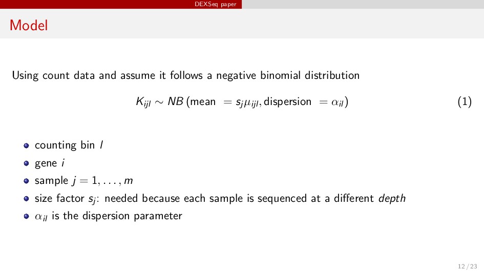
    a negative binomial distribution Kijl ∼ NB (mean = sj µijl , dispersion = αil ) (1) counting bin l gene i sample j = 1, . . . , m size factor sj : needed because each sample is sequenced at a different depth αil is the dispersion parameter 12 / 23

13. DEXSeq paper Poisson vs NB 10 Poisson GLM Outcome Y

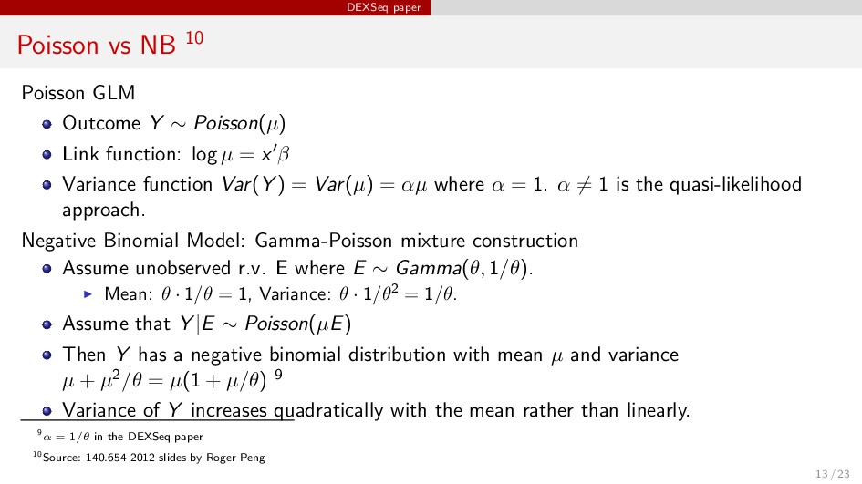
    ∼ Poisson(µ) Link function: log µ = x β Variance function Var(Y ) = Var(µ) = αµ where α = 1. α = 1 is the quasi-likelihood approach. Negative Binomial Model: Gamma-Poisson mixture construction Assume unobserved r.v. E where E ∼ Gamma(θ, 1/θ). Mean: θ · 1/θ = 1, Variance: θ · 1/θ2 = 1/θ. Assume that Y |E ∼ Poisson(µE) Then Y has a negative binomial distribution with mean µ and variance µ + µ2/θ = µ(1 + µ/θ) 9 Variance of Y increases quadratically with the mean rather than linearly. 9α = 1/θ in the DEXSeq paper 10Source: 140.654 2012 slides by Roger Peng 13 / 23

14. DEXSeq paper Main log-linear model log µijl = βG i

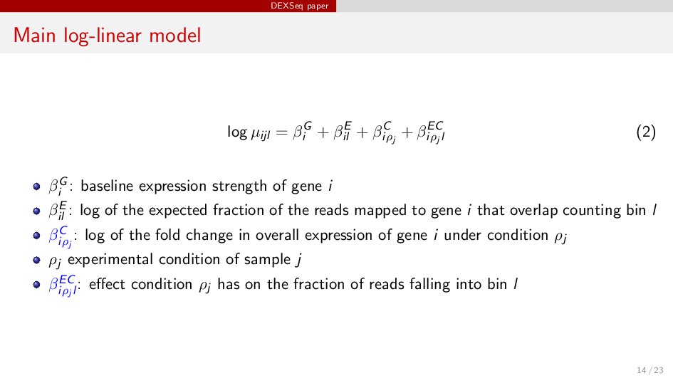
    + βE il + βC iρj + βEC iρj l (2) βG i : baseline expression strength of gene i βE il : log of the expected fraction of the reads mapped to gene i that overlap counting bin l βC iρj : log of the fold change in overall expression of gene i under condition ρj ρj experimental condition of sample j βEC iρj l : effect condition ρj has on the fraction of reads falling into bin l 14 / 23

15. DEXSeq paper Variability: gene expression + exon usage Var. in

    gene expression: when the total number of transcripts for a gene i differs from the expected value under ρj Var. in exon usage: using different exons or counting bins log µijl = βG i + βE il + βS ij + βEC iρj l (3) Change βC iρj by βS ij . Absorbs var. in gene expression. 15 / 23

16. DEXSeq paper Dispersion estimates 11 11Source: Anders, Reyes, Huber; Detecting

    differential usage of exons from RNA-seq data, 2012, Genome Research 16 / 23

17. DEXSeq paper Analysis of Deviance 12 Deviance D(ˆ β) =

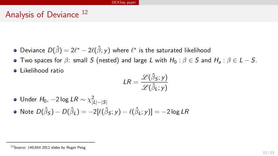
    2 ∗ − 2 (ˆ β; y) where ∗ is the saturated likelihood Two spaces for β: small S (nested) and large L with H0 : β ∈ S and Ha : β ∈ L − S. Likelihood ratio LR = L (ˆ βS ; y) L (ˆ βL; y) Under H0, −2 log LR ∼ χ2 |L|−|S| Note D(ˆ βS ) − D(ˆ βL) = −2[ (ˆ βS ; y) − (ˆ βL; y)] = −2 log LR 12Source: 140.654 2012 slides by Roger Peng 17 / 23

18. DEXSeq paper Testing for DEX: ANODEV Fit two models log

    µijl = βG i + βE il + βS ij (4) log µijl = βG i + βE il + βS ij + βEC iρj l δll (5) where δll = 1 if l = l 0 otherwise Then test using analysis of deviance (ANODEV) Control FDR by adjusting p-values using Benjamini-Hochberg’s method. 18 / 23

19. Results Finding DEX: knockdown of pasilla on Drosophila melanogaster example

    13 13Source http://www-huber.embl.de/pub/DEXSeq/analysis/brooksetal/ 19 / 23

20. Results Detection power depends on mean 14 14Source: reproduced with

    code from http://genome.cshlp.org/content/suppl/2012/08/20/gr.133744.111.DC1/Supp_II.html 20 / 23

21. Results Without considering biological variation 15 15Source http://www-huber.embl.de/pub/DEXSeq/analysis/brooksetal/ 21 /

    23

22. Results Interesting comparison Mock comparison: check for DEX between replicates

    from a control condition Used an FDR of 10% DEXSeq: 8 genes (159 in the real control vs treatment comparison) Cuffdiff v 1.3.0: 639 genes (37 in real comp.) This trend continues with other data sets. 22 / 23

23. Results Thanks! Main source: Anders, Reyes, Huber; Detecting differential usage

    of exons from RNA-seq data, 2012, Genome Research PMID: 22722343. 23 / 23