MLOS forecasting: IWLS call Friday 21 June 2013

Notes on the development of an experimental seasonal MLOS forecasting scheme for the Pacific Islands

Transcript

1. Introduction Data processing Methods Results Conclusion and recommendations Notes on the development of an experimental seasonal MLOS forecasting scheme for the Pacific Islands Nicolas Fauchereau 1,2 Scott Stephens 1 Nigel Goodhue 1 Rob Bell 1 Doug Ramsay 1 Nicolas.Fauchereau@niwa.co.nz 1NIWA Ltd., Auckland, New Zealand 2Oceanography Dept., University of Cape-Town, Cape-Town, South Africa June 21, 2013 1/19
2. Introduction Data processing Methods Results Conclusion and recommendations Table of contents 1 Introduction 2 Data processing Mean Level of the Sea anomalies (MLOS) Predictors sets Indices SST EOFs 3 Methods Regression Classification 4 Results 5 Conclusion and recommendations 2/19
3. Introduction Data processing Methods Results Conclusion and recommendations Introduction Rationale Set out in the “White Paper” High impact from sea level extremes Value in developing an “extreme sea-level calendar” Extreme tides + NTR (MLOS + “high frequency”) Goal Compared to existing PEAC scheme: Extend coverage to non-US affiliated Islands Frequency: every month for the coming 3 months (Island Climate Update) Performance of the model, type of forecast (probabilistic ?) 3/19
4. Introduction Data processing Methods Results Conclusion and recommendations Introduction Objective Provide recommendations: Data processing, predictand Choice of the set of predictors Statistical methods for prediction Operational Implementation Implementation For 3 Islands in the Pacific (presenting wide range of variability): ”Hindcast”: forecast for T+1 to 3 using information at T0 (e.g. May for June-August) Different predictors Different methods (state of the art Machine Learning) 4/19
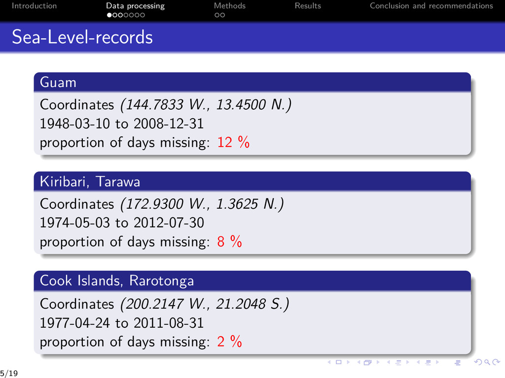
5. Introduction Data processing Methods Results Conclusion and recommendations Sea-Level-records Guam Coordinates (144.7833 W., 13.4500 N.) 1948-03-10 to 2008-12-31 proportion of days missing: 12 % Kiribari, Tarawa Coordinates (172.9300 W., 1.3625 N.) 1974-05-03 to 2012-07-30 proportion of days missing: 8 % Cook Islands, Rarotonga Coordinates (200.2147 W., 21.2048 S.) 1977-04-24 to 2011-08-31 proportion of days missing: 2 % 5/19
6. Introduction Data processing Methods Results Conclusion and recommendations Sea-Level-records Hourly sea-level (meters), tidal and high frequency component removed (Scott, Nigel, Rob) 1 Daily then Monthly averages 2 Series truncated before 1979-1-1 3 Climatology over 1979-2008 4 3-points running averages of monthly anomalies WRT climatology 1979 1984 1989 1994 1999 2004 2009 0.25 0.20 0.15 0.10 0.05 0.00 0.05 0.10 0.15 0.20 MLOS Seasonal Time-series Guam Kiribati Cooks 6/19
7. Introduction Data processing Methods Results Conclusion and recommendations Sea-Level-records 5 categories (”labels”) for classification algorithms: 1 ”well below” = (−inf, −0.15]: labelled ’WB’ 2 ”below” = (−0.15, −0.05]: labelled ’B’ 3 ”near-average” = (−0.05, +0.05]: labelled ’N’ 4 ”above” = (+0.05, +0.15]: labelled ’A’ 5 ”well-above” = (+0.15, inf): labelled ’WA’ Other approach is to used quantile-based categories 7/19
8. Introduction Data processing Methods Results Conclusion and recommendations Predictors sets Choice of the predictors set is dictated by: Relevance: Need to reflect plausible physical relationships between Ocean-Climate system and Sea-Level. Operational constraints: Must be available in near real time (within the first 5 days of Month 1 for forecast Season Month 1 - Month 3). 8/19
9. Introduction Data processing Methods Results Conclusion and recommendations Indices Indices of SST and Atmospheric variables, monthly time-scale: NINOS (1+2, 3.4, 3, 4): from CPC Southern Oscillation Index (SOI): calculated by NIWA, data from BoM El Nino Modoki Index (EMI): calculated from ERSST dataset Seasonal Cycle: (first 3 harmonics on MLOS climatology) Regional SST anomalies ... 9/19
10. Introduction Data processing Methods Results Conclusion and recommendations Indices: Regional SSTs Regression of SST anomalies on MLOS anomalies (lead 1 month) 10/19
11. Introduction Data processing Methods Results Conclusion and recommendations Sea-Surface-Temperatures EOFS EOF analysis of monthly anomalies of ERSST SSTs. 9 first Principal Components used as predictors 11/19
12. Introduction Data processing Methods Results Conclusion and recommendations Methods Machine Learning Regression: continuous dependent variable Classification: discrete, categorical dependent variable Regression 1 Generalized Linear Models: Extension of linear regression for distributions of the exponential family (Normal, Poisson, Binomial, Multinomial, etc) Ordinary Least Square (Linear Regression) Penalized Least Square (Ridge Regression, LARS, LASSO) Logistic Regression 2 Multivariate Adaptative Regression Splines (MARS): Non-parametric multivariate regression method Models non-linearities and interactions between predictors Similarities with stepwise regression and CART (Classification And Regression Trees: recursive partitioning) 12/19
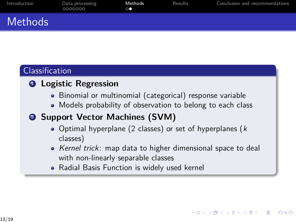
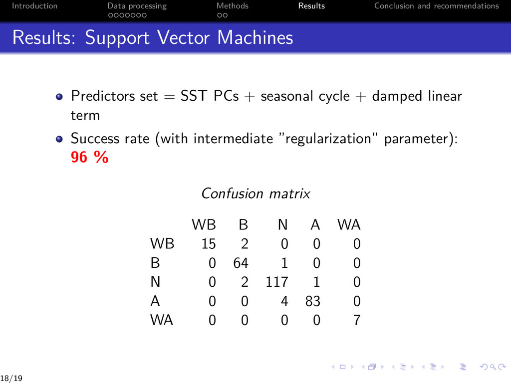
13. Introduction Data processing Methods Results Conclusion and recommendations Methods Classification 1 Logistic Regression Binomial or multinomial (categorical) response variable Models probability of observation to belong to each class 2 Support Vector Machines (SVM) Optimal hyperplane (2 classes) or set of hyperplanes (k classes) Kernel trick: map data to higher dimensional space to deal with non-linearly separable classes Radial Basis Function is widely used kernel 13/19
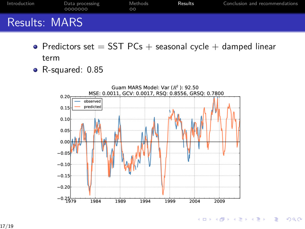
14. Introduction Data processing Methods Results Conclusion and recommendations Approach All the methods referred to above are tested in turn, using successively the Indices and the SST EOFs set as predictors Applied to Guam, Kiribati and Cooks ”Best” Model selected using objective measures (i.e. R-squared) + cross-validation + expert judgment Results for Guam only presented in details 14/19
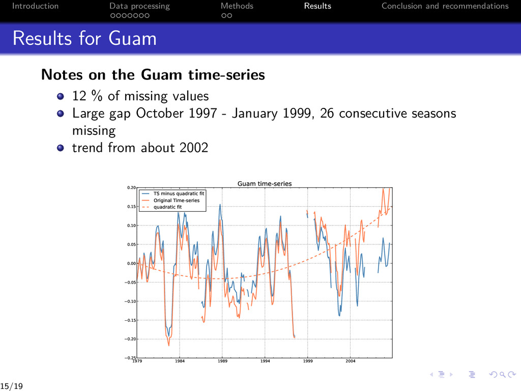
15. Introduction Data processing Methods Results Conclusion and recommendations Results for Guam Notes on the Guam time-series 12 % of missing values Large gap October 1997 - January 1999, 26 consecutive seasons missing trend from about 2002 1979 1984 1989 1994 1999 2004 −0.25 −0.20 −0.15 −0.10 −0.05 0.00 0.05 0.10 0.15 0.20 Guam time-series TS minus quadratic fit Original Time-series quadratic fit 15/19
16. Introduction Data processing Methods Results Conclusion and recommendations Results: Logistic regression (Multinomial) Predictors set = SST PCs + seasonal cycle Success rate: 66.2 % (random: 20 %) Probabilistic forecast well-below below normal above well-above 0 1 2 3 4 5 6 7 8 9 Time (seasons) Exemple of a Multinomial Logistic regression probabilistic forecast 0.0 0.1 0.2 0.3 0.4 0.5 0.6 0.7 0.8 Prob. 16/19
17. Introduction Data processing Methods Results Conclusion and recommendations Results: MARS Predictors set = SST PCs + seasonal cycle + damped linear term R-squared: 0.85 1979 1984 1989 1994 1999 2004 2009 0.25 0.20 0.15 0.10 0.05 0.00 0.05 0.10 0.15 0.20 Guam MARS Model: Var (R2 ): 92.50 MSE: 0.0011, GCV: 0.0017, RSQ: 0.8556, GRSQ: 0.7800 observed predicted 17/19
18. Introduction Data processing Methods Results Conclusion and recommendations Results: Support Vector Machines Predictors set = SST PCs + seasonal cycle + damped linear term Success rate (with intermediate ”regularization” parameter): 96 % Confusion matrix WB B N A WA WB 15 2 0 0 0 B 0 64 1 0 0 N 0 2 117 1 0 A 0 0 4 83 0 WA 0 0 0 0 7 18/19
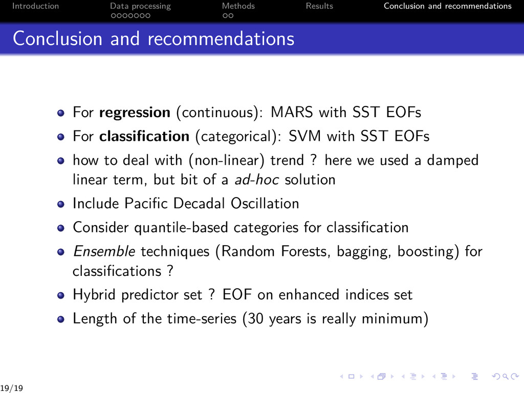
19. Introduction Data processing Methods Results Conclusion and recommendations Conclusion and recommendations For regression (continuous): MARS with SST EOFs For classification (categorical): SVM with SST EOFs how to deal with (non-linear) trend ? here we used a damped linear term, but bit of a ad-hoc solution Include Pacific Decadal Oscillation Consider quantile-based categories for classification Ensemble techniques (Random Forests, bagging, boosting) for classifications ? Hybrid predictor set ? EOF on enhanced indices set Length of the time-series (30 years is really minimum) 19/19