Introduction to ggplot2

Transcript

1. Introduction to ggplot2 fukuoka.R #13 @nonki1974 April 7, 2019
2. ggplot2 package → Wilkinson(2005) による “Grammar of Graphics” の R への実 装 → データの可視化のための一貫した文法と洗練された出力を提 供 → 開発者は dplyr と同じ Hadley Wickham 2
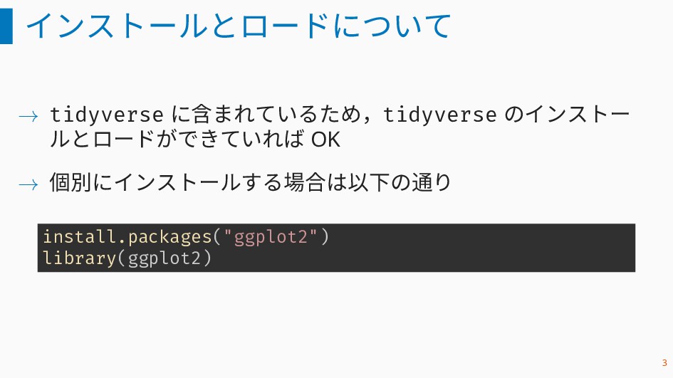
3. インストールとロードについて → tidyverse に含まれているため，tidyverse のインストー ルとロードができていれば OK → 個別にインストールする場合は以下の通り install.packages("ggplot2") library(ggplot2) 3
4. 本資料におけるバージョン packageVersion("ggplot2") ## [1] '3.1.0' 4
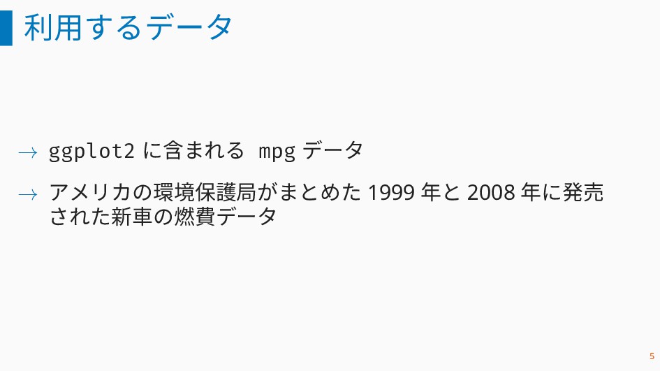
5. 利用するデータ → ggplot2 に含まれる mpg データ → アメリカの環境保護局がまとめた 1999 年と 2008 年に発売 された新車の燃費データ 5
6. mpg データ mpg[1:6, 2:8] %>% knitr ::kable(booktabs = TRUE) model displ year cyl trans drv cty a4 1.8 1999 4 auto(l5) f 18 a4 1.8 1999 4 manual(m5) f 21 a4 2.0 2008 4 manual(m6) f 20 a4 2.0 2008 4 auto(av) f 21 a4 2.8 1999 6 auto(l5) f 16 a4 2.8 1999 6 manual(m5) f 18 6
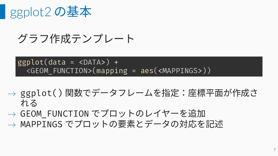
7. ggplot2 の基本 グラフ作成テンプレート ggplot(data = <DATA>) + <GEOM_FUNCTION>(mapping = aes(<MAPPINGS>)) → ggplot() 関数でデータフレームを指定：座標平面が作成さ れる → GEOM_FUNCTION でプロットのレイヤーを追加 → MAPPINGS でプロットの要素とデータの対応を記述 7
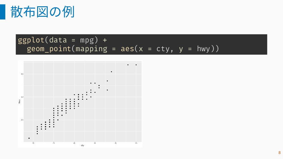
8. 散布図の例 ggplot(data = mpg) + geom_point(mapping = aes(x = cty, y = hwy)) 20 30 40 10 15 20 25 30 35 cty hwy 8
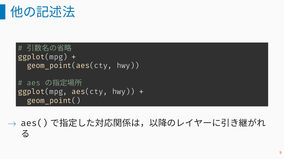
9. 他の記述法 # 引数名の省略 ggplot(mpg) + geom_point(aes(cty, hwy)) # aes の指定場所 ggplot(mpg, aes(cty, hwy)) + geom_point() → aes() で指定した対応関係は，以降のレイヤーに引き継がれ る 9
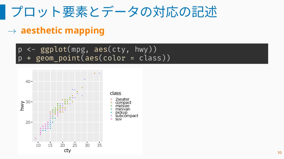
10. プロット要素とデータの対応の記述 → aesthetic mapping p <- ggplot(mpg, aes(cty, hwy)) p + geom_point(aes(color = class)) 20 30 40 10 15 20 25 30 35 cty hwy class 2seater compact midsize minivan pickup subcompact suv 10
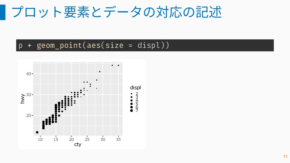
11. プロット要素とデータの対応の記述 p + geom_point(aes(size = displ)) 20 30 40 10 15 20 25 30 35 cty hwy displ 2 3 4 5 6 7 11
12. 1 変数に対するプロット 12
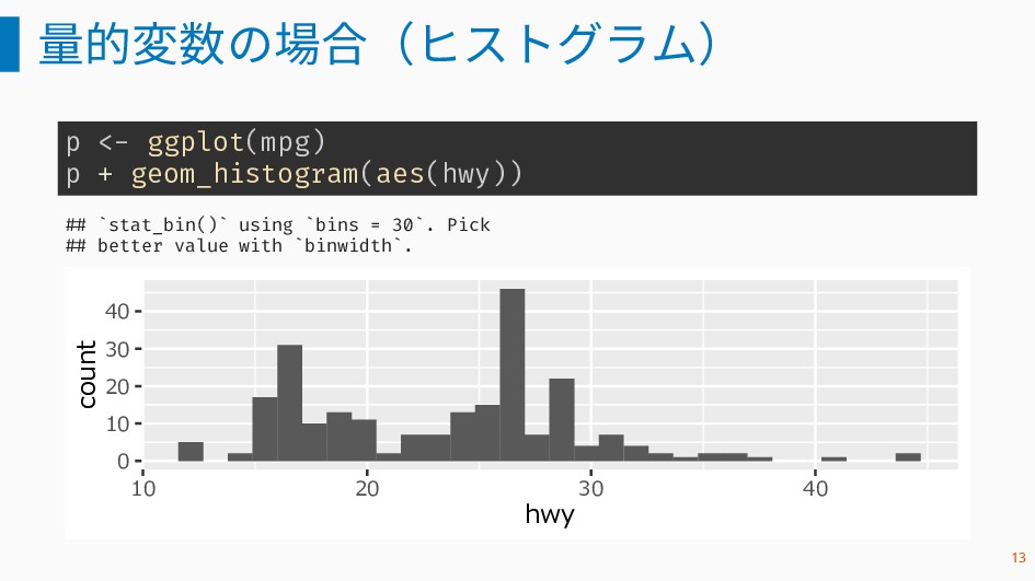
13. 量的変数の場合（ヒストグラム） p <- ggplot(mpg) p + geom_histogram(aes(hwy)) ## `stat_bin()` using `bins = 30`. Pick ## better value with `binwidth`. 0 10 20 30 40 10 20 30 40 hwy count 13
14. 色の指定 p + geom_histogram(aes(hwy), binwidth = 2, fill = "cadetblue", color = "black") 0 10 20 30 40 10 20 30 40 hwy count 14
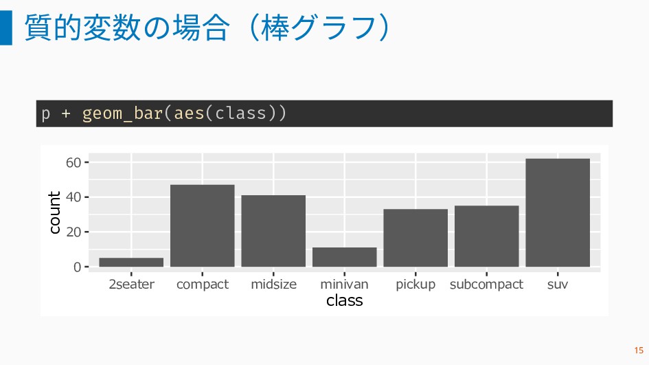
15. 質的変数の場合（棒グラフ） p + geom_bar(aes(class)) 0 20 40 60 2seater compact midsize minivan pickup subcompact suv class count 15
16. 降順にソート forcats ::fct_infreq()：因子型の水準の順序を値の出現 頻度順に並べ替える p + geom_bar(aes(fct_infreq(class))) + xlab("class") 0 20 40 60 suv compact midsize subcompact pickup minivan 2seater class count 16
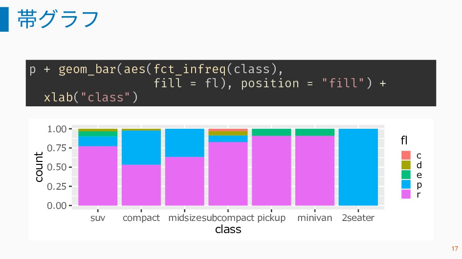
17. 帯グラフ p + geom_bar(aes(fct_infreq(class), fill = fl), position = "fill") + xlab("class") 0.00 0.25 0.50 0.75 1.00 suv compact midsizesubcompact pickup minivan 2seater class count fl c d e p r 17
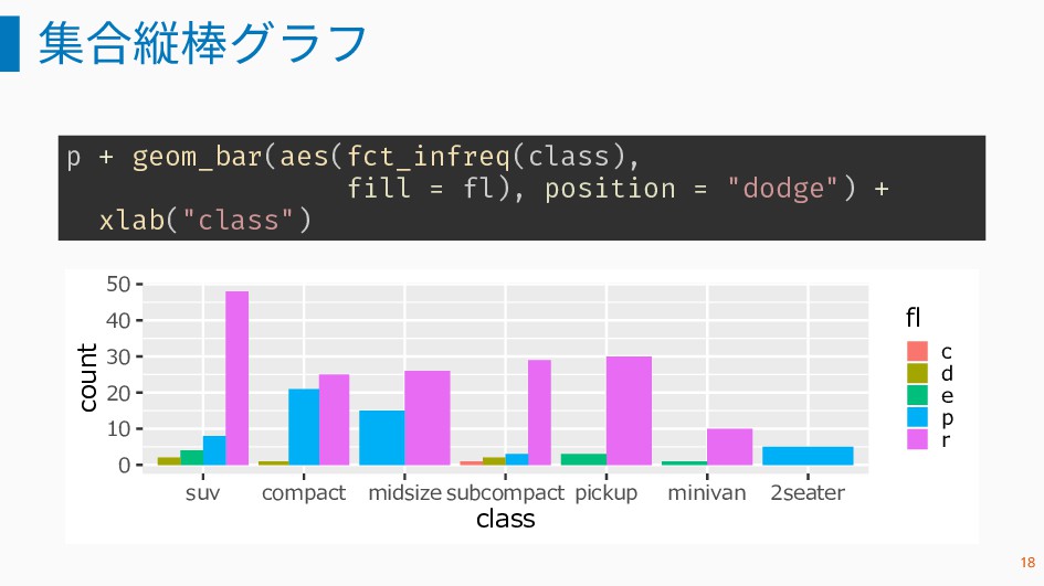
18. 集合縦棒グラフ p + geom_bar(aes(fct_infreq(class), fill = fl), position = "dodge") + xlab("class") 0 10 20 30 40 50 suv compact midsize subcompact pickup minivan 2seater class count fl c d e p r 18
19. 2 変数に対するプロット 19
20. x: 量的変数，y: 量的変数の場合（散布図） p + geom_point(aes(cty, hwy)) + geom_smooth(method = "lm") 20 30 40 50 10 15 20 25 30 35 cty hwy 20
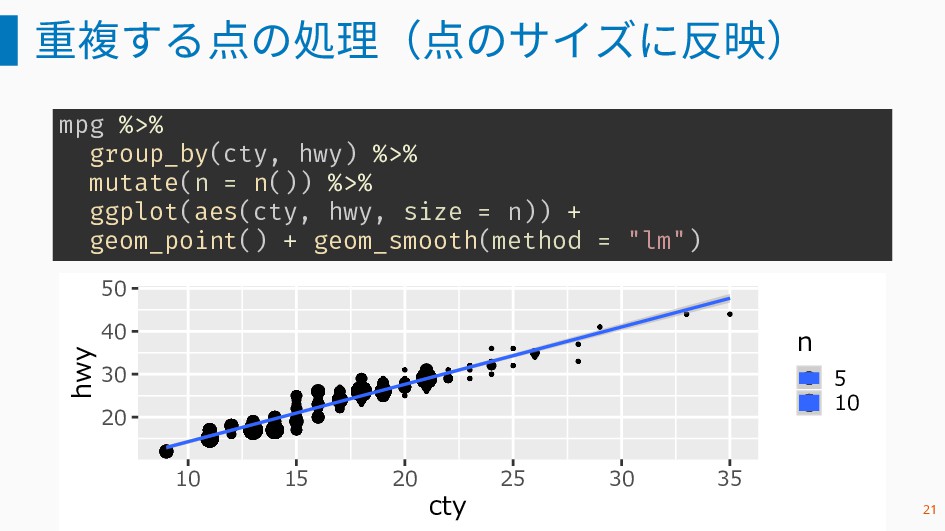
21. 重複する点の処理（点のサイズに反映） mpg %>% group_by(cty, hwy) %>% mutate(n = n()) %>% ggplot(aes(cty, hwy, size = n)) + geom_point() + geom_smooth(method = "lm") 20 30 40 50 10 15 20 25 30 35 cty hwy n 5 10 21
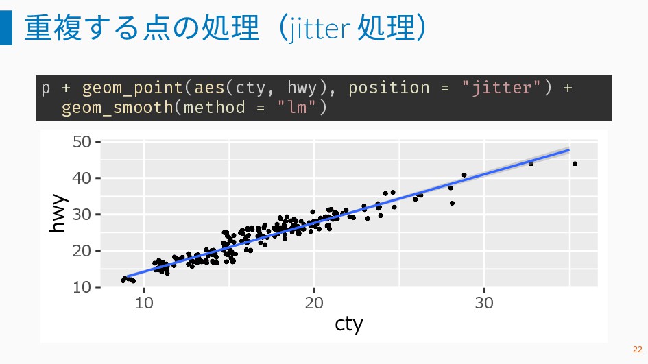
22. 重複する点の処理（jitter 処理） p + geom_point(aes(cty, hwy), position = "jitter") + geom_smooth(method = "lm") 10 20 30 40 50 10 20 30 cty hwy 22
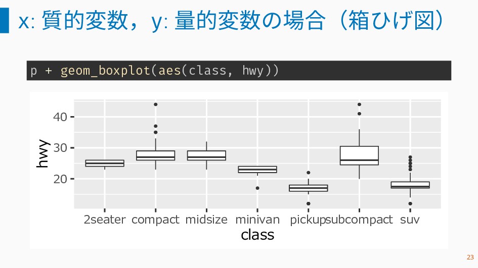
23. x: 質的変数，y: 量的変数の場合（箱ひげ図） p + geom_boxplot(aes(class, hwy)) 20 30 40 2seater compact midsize minivan pickupsubcompact suv class hwy 23
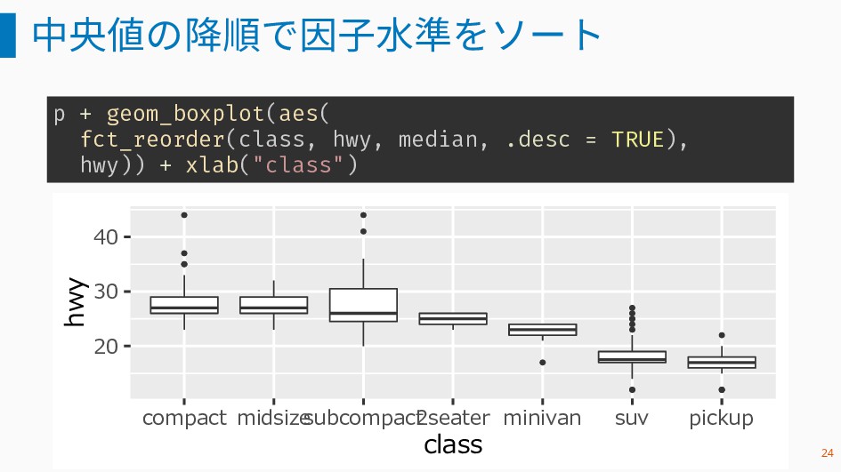
24. 中央値の降順で因子水準をソート p + geom_boxplot(aes( fct_reorder(class, hwy, median, .desc = TRUE), hwy)) + xlab("class") 20 30 40 compact midsize subcompact 2seater minivan suv pickup class hwy 24
25. 質的変数による プロット分割 （Facetting） 25
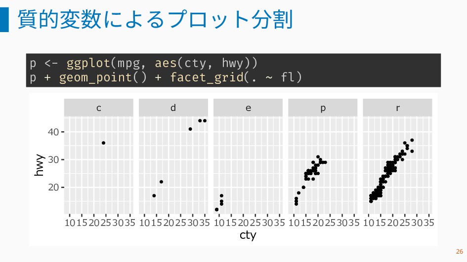
26. 質的変数によるプロット分割 p <- ggplot(mpg, aes(cty, hwy)) p + geom_point() + facet_grid(. ~ fl) c d e p r 101520253035 101520253035 101520253035 101520253035 101520253035 20 30 40 cty hwy 26
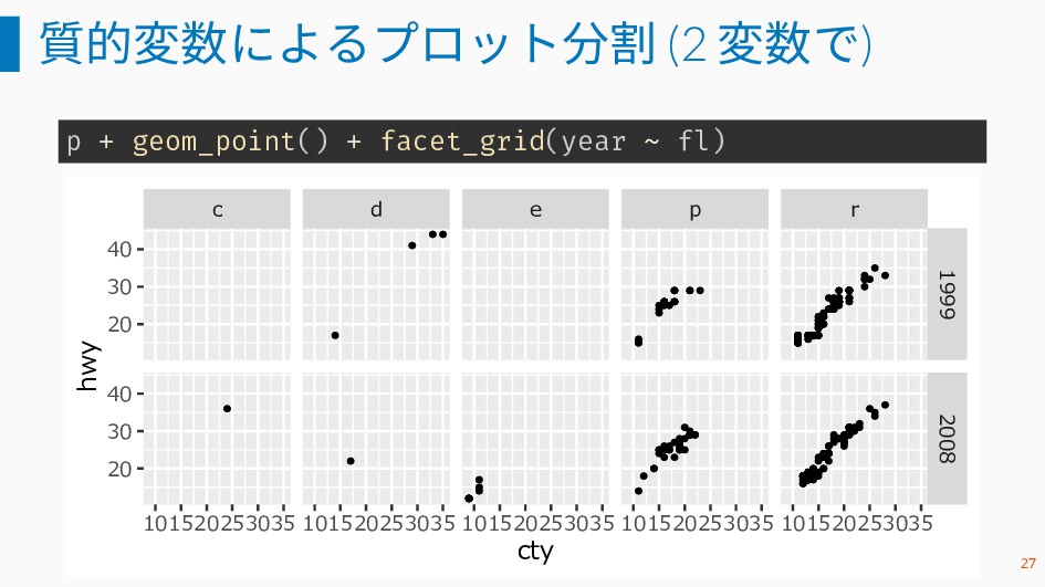
27. 質的変数によるプロット分割 (2 変数で) p + geom_point() + facet_grid(year ~ fl) c d e p r 1999 2008 101520253035 101520253035 101520253035 101520253035 101520253035 20 30 40 20 30 40 cty hwy 27
28. 集計表に対する棒グラフ 28
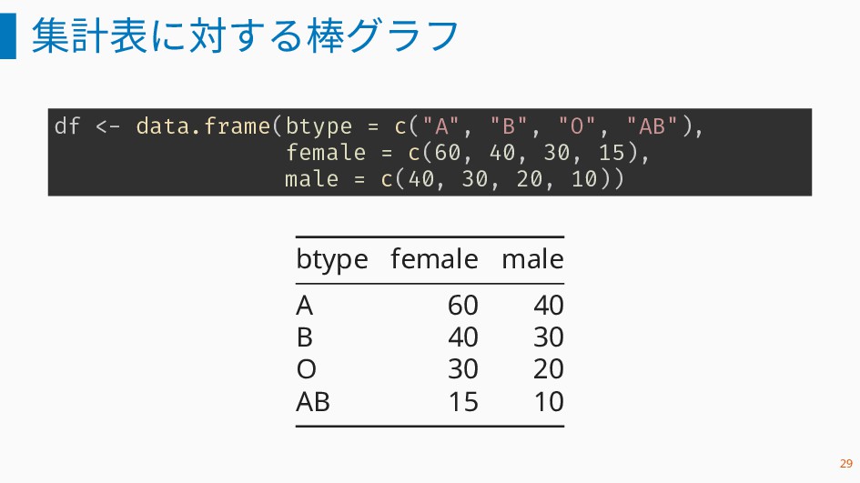
29. 集計表に対する棒グラフ df <- data.frame(btype = c("A", "B", "O", "AB"), female = c(60, 40, 30, 15), male = c(40, 30, 20, 10)) btype female male A 60 40 B 40 30 O 30 20 AB 15 10 29
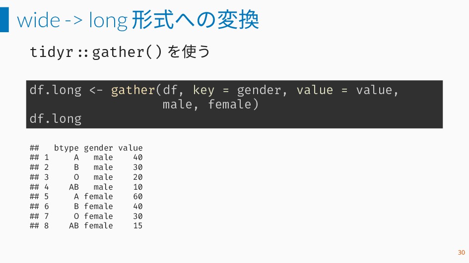
30. wide -> long 形式への変換 tidyr ::gather() を使う df.long <- gather(df, key = gender, value = value, male, female) df.long ## btype gender value ## 1 A male 40 ## 2 B male 30 ## 3 O male 20 ## 4 AB male 10 ## 5 A female 60 ## 6 B female 40 ## 7 O female 30 ## 8 AB female 15 30
31. 棒グラフの作成 stat = "identity" を指定 ggplot(df.long, aes(fct_reorder(btype, value, sum, .desc = TRUE), val fill = gender)) + xlab("btype") + geom_bar(stat = "identity", position = "dodge") 0 20 40 60 A B O AB btype value gender female male 31
32. 外見の調整 32
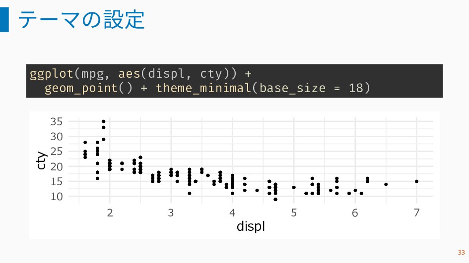
33. テーマの設定 ggplot(mpg, aes(displ, cty)) + geom_point() + theme_minimal(base_size = 18) 10 15 20 25 30 35 2 3 4 5 6 7 displ cty 33
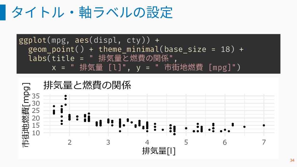
34. タイトル・軸ラベルの設定 ggplot(mpg, aes(displ, cty)) + geom_point() + theme_minimal(base_size = 18) + labs(title = " 排気量と燃費の関係", x = " 排気量 [l]", y = " 市街地燃費 [mpg]") 10 15 20 25 30 35 2 3 4 5 6 7 排気量[l] 市街地燃費[mpg] 排気量と燃費の関係 34
35. GGally パッケージの利用 35
36. インストールとパッケージの読み込み install.packages("GGally") library(GGally) ## ## Attaching package: 'GGally' ## The following object is masked from 'package:dplyr': ## ## nasa 36
37. 平行座標プロット ggparcoord(mpg, columns = c(4, 3, 8, 9), groupColumn = "class") + theme_minimal(base_size = 18) -2 0 2 4 year displ cty hwy variable value class 2seater compact midsize minivan pickup subcompact suv 37
38. 相関行列の可視化（データの読み込み） nba <- read.csv( "http: //datasets.flowingdata.com/ppg2008.csv") 38
39. 相関行列の可視化 ggcorr(nba[,-1]) G MIN PTS FGM FGA FGP FTM FTA FTP X3PM X3PA X3PP ORB DRB TRB AST STL BLK TO PF -1.0 -0.5 0.0 0.5 1.0 39
40. 相関行列の可視化（オプション設定） ggcorr(nba[,-1], label = TRUE, label_size = 1, label_round = 2, label_alpha = TRUE) 0.19 0.06 0.04 -0.06 0.18 -0.01 0.01 0.04 0.14 0.11 0.12 0.05 0.12 0.1 0.14 -0.03 0.13 -0.05 -0.03 0.4 0.3 0.41 -0.22 0.27 0.18 0.22 0.13 0.13 0.11 -0.07 0.05 0.01 0.28 0.33 -0.07 0.32 -0.39 0.85 0.83 0.07 0.67 0.61 0.03 0.03 0.04 0.01 0.01 0.25 0.17 0.22 0.36 0.24 0.34 -0.15 0.87 0.27 0.28 0.29 -0.13 -0.23 -0.22 -0.09 0.23 0.38 0.34 0.11 0.22 0.33 0.14 -0.12 -0.23 0.25 0.17 0.11 0.1 0.14 -0.02 -0.1 0.08 0.02 0.17 0.33 0 0.16 -0.24 0.07 0.25 -0.52 -0.64 -0.67 -0.16 0.66 0.61 0.65 -0.16 -0.23 0.68 -0.02 0.26 0.95 -0.03 -0.14 -0.13 -0.02 0.01 0.24 0.17 0.23 0.3 0.23 0.54 0.03 -0.33 -0.29 -0.27 -0.21 0.21 0.4 0.34 0.16 0.26 0.42 0.52 0.12 0.53 0.5 0.6 -0.62 -0.53 -0.58 0.2 0.07 -0.54 -0.02 -0.25 0.99 0.31 -0.64 -0.59 -0.63 0.09 0.16 -0.49 -0.11 -0.25 0.28 -0.65 -0.61 -0.65 0.16 0.24 -0.52 -0.06 -0.27 -0.31 -0.25 -0.28 0.04 -0.04 -0.26 0.1 -0.07 0.85 0.93 -0.46 -0.33 0.74 -0.13 0.41 0.98 -0.4 -0.27 0.77 0.03 0.43 -0.43 -0.3 0.79 -0.03 0.43 0.62 -0.32 0.5 -0.43 -0.26 0.45 -0.19 0.12 0.37 0.07 G MIN PTS FGM FGA FGP FTM FTA FTP X3PM X3PA X3PP ORB DRB TRB AST STL BLK TO PF -1.0 -0.5 0.0 0.5 1.0 40