Introduction to dplyr

Transcript

1. Introduction to dplyr fukuoka.R #13 @nonki1974 April 6, 2019
2. データの前処理と可視化 → データの要約と可視化はデータ分析に欠かせない → 要約と可視化を行うためには，データがきれいな形であるこ とが前提 → きれいな形にする一連の処理 => 前処理 2
3. サンプルデータ → nycflights13 パッケージのデータを使う # パッケージのインストール install.packages("nycflights13") → tidyverse パッケージを入れていない場合は以下も実行 # パッケージのインストール install.packages("tidyverse") 3
4. ライブラリの読み込み library(tidyverse) ## -- Attaching packages ----------------------------------------------------- tidyverse ## v ggplot2 3.1.0 v purrr 0.3.0 ## v tibble 2.0.1 v dplyr 0.8.0.1 ## v tidyr 0.8.2 v stringr 1.3.1 ## v readr 1.3.1 v forcats 0.3.0 ## -- Conflicts -------------------------------------------------------- tidyverse_confli ## x dplyr ::filter() masks stats ::filter() ## x dplyr ::lag() masks stats ::lag() library(nycflights13) 4
5. nycflights13 flights ## # A tibble: 336,776 x 19 ## year month day dep_time ## <int> <int> <int> <int> ## 1 2013 1 1 517 ## 2 2013 1 1 533 ## 3 2013 1 1 542 ## 4 2013 1 1 544 ## 5 2013 1 1 554 ## 6 2013 1 1 554 ## 7 2013 1 1 555 ## 8 2013 1 1 557 ## 9 2013 1 1 557 ## 10 2013 1 1 558 ## # ... with 336,766 more rows, and 15 ## # more variables: ## # sched_dep_time <int>, ## # dep_delay <dbl>, arr_time <int>, ## # sched_arr_time <int>, ## # arr_delay <dbl>, carrier <chr>, 5
6. nycflights13 → 2013 年にニューヨークから出発した 336776 便のフライト データ → データフレームの拡張である tibble 6
7. dplyr による前処理 7
8. dplyr package dplyr ”a grammar of data manipulation” → データ操作のための基本操作（verb）を R で実装 → 高速に実行できる → データがデータベースに格納されていても同じ関数で実行で きる 8
9. 今回扱う verb の一覧 verb 機能 filter() 与えた条件に合致する行を抽出 select() 指定した列のみを抽出 arrange() 行を指定した列の値に基づいて並べ替える mutate() 新しい変数を作成する summarize() 変数の要約（平均など）を計算する 9
10. verb 共通の性質 → 第 1 引数はデータフレーム → 続く引数はデータフレームに何をするか記述し，引用符なし の変数名をとる → 結果は新たなデータフレーム 10
11. サンプルデータの作成 df <- data.frame( color = c("blue", "black", "blue", "blue", "black"), value = 1:5 ) df ## color value ## 1 blue 1 ## 2 black 2 ## 3 blue 3 ## 4 blue 4 ## 5 black 5 11
12. 与えた条件に合致する行を 抽出:filter() 12
13. 与えた条件に合致する行を抽出:filter() 第 2 引数以降で指定した条件に合致する行のみを抽出する。 filter(df, color "blue") ## color value ## 1 blue 1 ## 2 blue 3 ## 3 blue 4 変数 value が 1 もしくは 4 の行のみを抽出する filter(df, value %in% c(1, 4)) ## color value ## 1 blue 1 ## 2 blue 4 13
14. 与えた条件に合致する行を抽出:filter() color が blue で value が 3 未満の行のみを抽出する filter(df, color "blue" & value 3) ## color value ## 1 blue 1 ## 2 blue 3 14
15. nycflights13 の例 出発時の遅延は少なくとも 1 時間を超えたが，運行では 30 分 以上取り返したフライトを抽出 filter(flights, dep_delay > 60 & arr_delay dep_delay - 30) ## # A tibble: 2,046 x 19 ## year month day dep_time ## <int> <int> <int> <int> ## 1 2013 1 1 1716 ## 2 2013 1 1 2205 ## 3 2013 1 1 2326 ## 4 2013 1 3 1503 ## 5 2013 1 3 1821 ## 6 2013 1 3 1839 ## 7 2013 1 3 1850 ## 8 2013 1 3 1923 ## 9 2013 1 3 1941 ## 10 2013 1 3 1950 15
16. 指定した列のみを抽 出:select() 16
17. 指定した列のみを抽出:select() df から変数 color を抽出 select(df, color) ## color ## 1 blue ## 2 black ## 3 blue ## 4 blue ## 5 black df から変数 color を削除 select(df, -color) ## value ## 1 1 ## 2 2 ## 3 3 17
18. 指定した列のみを抽出:select() フライトデータから year と day の間にある変数を全て選 ぶ select(flights, year:day) ## # A tibble: 336,776 x 3 ## year month day ## <int> <int> <int> ## 1 2013 1 1 ## 2 2013 1 1 ## 3 2013 1 1 ## 4 2013 1 1 ## 5 2013 1 1 ## 6 2013 1 1 ## 7 2013 1 1 ## 8 2013 1 1 ## 9 2013 1 1 ## 10 2013 1 1 ## # ... with 336,766 more rows 18
19. ヘルパー関数の利用 → start_with("abc") は abc で始まる名前にマッチする → end_with("xyz") は xyz で終わる名前にマッチする → contains("ijk") は ijk を含む名前にマッチする → num_range("x", 1:3) は x1,x2,x3 にマッチする 19
20. ヘルパー関数の利用例 select(flights, contains("time")) ## # A tibble: 336,776 x 6 ## dep_time sched_dep_time arr_time ## <int> <int> <int> ## 1 517 515 830 ## 2 533 529 850 ## 3 542 540 923 ## 4 544 545 1004 ## 5 554 600 812 ## 6 554 558 740 ## 7 555 600 913 ## 8 557 600 709 ## 9 557 600 838 ## 10 558 600 753 ## # ... with 336,766 more rows, and 3 ## # more variables: ## # sched_arr_time <int>, ## # air_time <dbl>, time_hour <dttm> 20
21. 並べ替え:arrange() 21
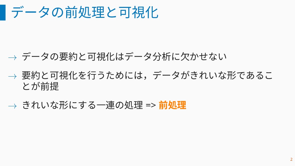
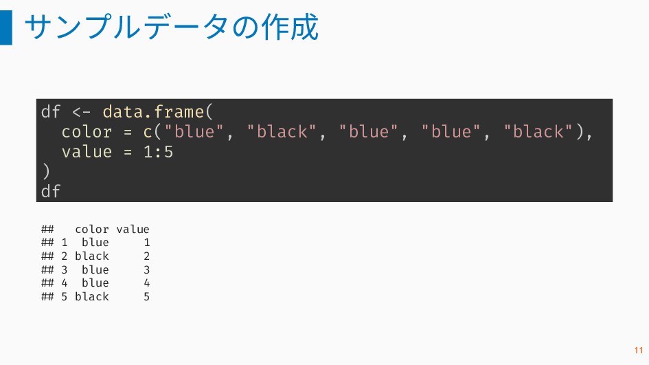
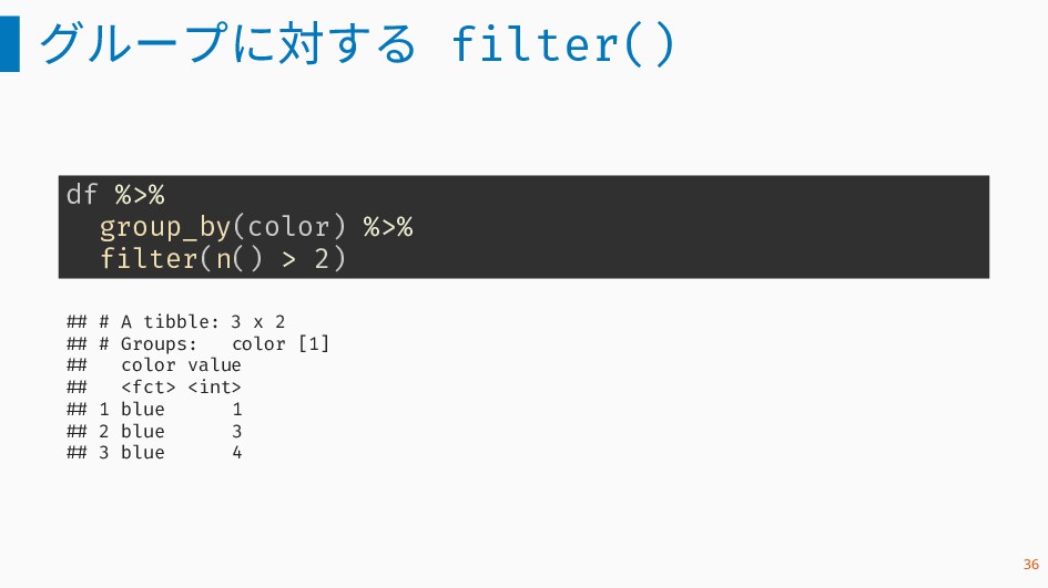
22. 並べ替え:arrange() color のアルファベット順に昇順でソート arrange(df, color) ## color value ## 1 black 2 ## 2 black 5 ## 3 blue 1 ## 4 blue 3 ## 5 blue 4 desc() 関数を使って value の値で降順にソート arrange(df, desc(value)) ## color value ## 1 black 5 ## 2 blue 4 ## 3 blue 3 22
23. 新しい変数を作成す る:mutate() 23
24. 新しい変数を作成する:mutate() mutate(df, double = 2*value) ## color value double ## 1 blue 1 2 ## 2 black 2 4 ## 3 blue 3 6 ## 4 blue 4 8 ## 5 black 5 10 mutate(df, double = 2*value, quad = 2*double) ## color value double quad ## 1 blue 1 2 4 ## 2 black 2 4 8 ## 3 blue 3 6 12 ## 4 blue 4 8 16 ## 5 black 5 10 20 24
25. 新しい変数を作成する:mutate() flights_sml <- select(flights, air_time, distance) mutate(flights_sml, air_hours = air_time / 60, dist_km = distance * 1.609) ## # A tibble: 336,776 x 4 ## air_time distance air_hours dist_km ## <dbl> <dbl> <dbl> <dbl> ## 1 227 1400 3.78 2253. ## 2 227 1416 3.78 2278. ## 3 160 1089 2.67 1752. ## 4 183 1576 3.05 2536. ## 5 116 762 1.93 1226. ## 6 150 719 2.5 1157. ## 7 158 1065 2.63 1714. ## 8 53 229 0.883 368. ## 9 140 944 2.33 1519. ## 10 138 733 2.3 1179. ## # ... with 336,766 more rows 25
26. グループごとの要約 group_by() summrize() 26
27. グループごとの要約 全体の要約をしたい場合 summarize(df, total = sum(value)) ## total ## 1 15 27
28. グループごとの要約 グループごとに要約したい場合，group_by() 関数で，グル ープの情報をデータに付加してから summarize() で要約す る。 by_color <- group_by(df, color) summarise(by_color, total = sum(value)) ## # A tibble: 2 x 2 ## color total ## <fct> <int> ## 1 black 7 ## 2 blue 8 28
29. グループごとの要約 by_color にはグループ情報が付加されている。 by_color ## # A tibble: 5 x 2 ## # Groups: color [2] ## color value ## <fct> <int> ## 1 blue 1 ## 2 black 2 ## 3 blue 3 ## 4 blue 4 ## 5 black 5 29
30. グループごとの要約 複数列でグループ化できる by_date <- group_by(flights, year, month, day) summarise(by_date, count = n()) ## # A tibble: 365 x 4 ## # Groups: year, month [12] ## year month day count ## <int> <int> <int> <int> ## 1 2013 1 1 842 ## 2 2013 1 2 943 ## 3 2013 1 3 914 ## 4 2013 1 4 915 ## 5 2013 1 5 720 ## 6 2013 1 6 832 ## 7 2013 1 7 933 ## 8 2013 1 8 899 ## 9 2013 1 9 902 ## 10 2013 1 10 932 ## # ... with 355 more rows 30
31. パイプ演算子 31
32. パイプ hourly_delay <- filter( summarize( group_by( filter( flights, !is.na(dep_delay) ), year, month, day, hour ), delay = mean(dep_delay), n = n() ), n > 10 ) 32
33. パイプ パイプ演算子%>% を使えば x %>% f(y) と記述すれば f(x, y) が実行される。連続した verb をパイプ演算子で接続できる。 33
34. パイプ RStudio では，パイプ演算子をショートカット [Ctrl]+[Shift]+[M] で入力できる。 hourly_delay <- flights %>% filter(!is.na(dep_delay)) %>% group_by(year, month, day, hour) %>% summarize(delay = mean(dep_delay), n = n()) %>% filter(n > 10) 34
35. グループに対する filter() mutate() 35
36. グループに対する filter() df %>% group_by(color) %>% filter(n() > 2) ## # A tibble: 3 x 2 ## # Groups: color [1] ## color value ## <fct> <int> ## 1 blue 1 ## 2 blue 3 ## 3 blue 4 36
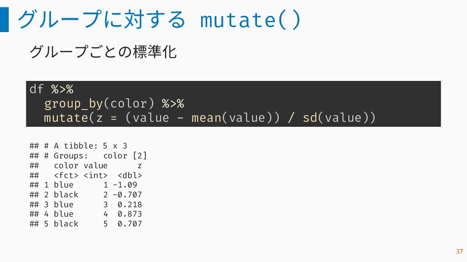
37. グループに対する mutate() グループごとの標準化 df %>% group_by(color) %>% mutate(z = (value - mean(value)) / sd(value)) ## # A tibble: 5 x 3 ## # Groups: color [2] ## color value z ## <fct> <int> <dbl> ## 1 blue 1 -1.09 ## 2 black 2 -0.707 ## 3 blue 3 0.218 ## 4 blue 4 0.873 ## 5 black 5 0.707 37
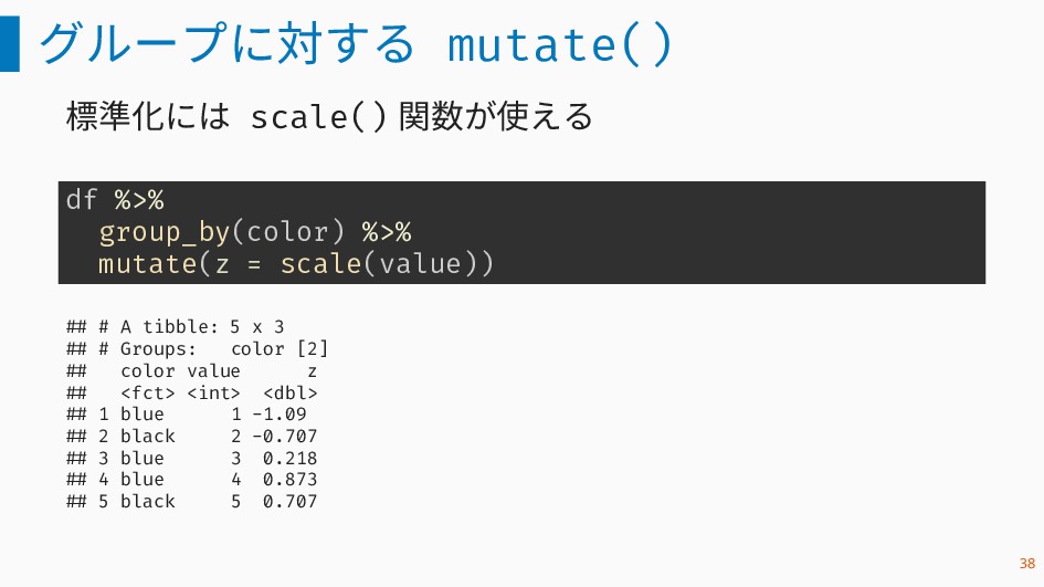
38. グループに対する mutate() 標準化には scale() 関数が使える df %>% group_by(color) %>% mutate(z = scale(value)) ## # A tibble: 5 x 3 ## # Groups: color [2] ## color value z ## <fct> <int> <dbl> ## 1 blue 1 -1.09 ## 2 black 2 -0.707 ## 3 blue 3 0.218 ## 4 blue 4 0.873 ## 5 black 5 0.707 38
39. ウインドウ関数 グループ内の順位や累積分布を出力する関数 x <- c(1, 1, 2, 2, 2) # グループ内での出現順序 row_number(x) ## [1] 1 2 3 4 5 # 昇順に並べた際の順序（ギャップ有り） min_rank(x) ## [1] 1 1 3 3 3 # 昇順に並べた際の順序（ギャップ無し） dense_rank(x) 39
40. ウインドウ関数 # 累積分布 cume_dist(x) ## [1] 0.4 0.4 1.0 1.0 1.0 # min_rank を [0,1] とした場合の値 percent_rank(x) ## [1] 0.0 0.0 0.5 0.5 0.5 40
41. テーブルの結合 41
42. サンプルデータ x <- data.frame( name = c("John", "Paul", "George", "Ringo", "Stuart", "Pete"), instrument = c("guitar", "bass", "guitar", "drums", "bass", "drums"), stringsAsFactors = FALSE ) y <- data.frame( name = c("John", "Paul", "George", "Ringo", "Brian"), band = c("TRUE", "TRUE", "TRUE", "TRUE", "FALSE"), stringsAsFactors = FALSE ) 42
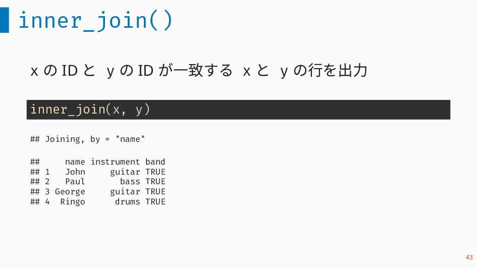
43. inner_join() x の ID と y の ID が一致する x と y の行を出力 inner_join(x, y) ## Joining, by = "name" ## name instrument band ## 1 John guitar TRUE ## 2 Paul bass TRUE ## 3 George guitar TRUE ## 4 Ringo drums TRUE 43
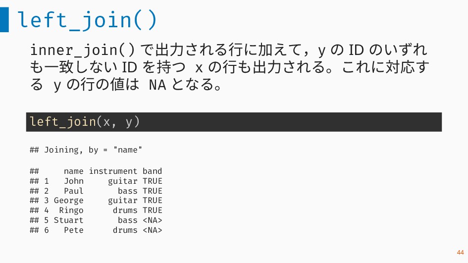
44. left_join() inner_join() で出力される行に加えて，y の ID のいずれ も一致しない ID を持つ x の行も出力される。これに対応す る y の行の値は NA となる。 left_join(x, y) ## Joining, by = "name" ## name instrument band ## 1 John guitar TRUE ## 2 Paul bass TRUE ## 3 George guitar TRUE ## 4 Ringo drums TRUE ## 5 Stuart bass <NA> ## 6 Pete drums <NA> 44
45. 結合するための ID を指定する デフォルトでは，2 つのテーブルで同じ名前を持つ変数（複数 ある場合は変数の組）が結合のための ID として用いられる。 異なる名前を持つ変数で結合する場合や，ID として用いる変 数を指定したい場合は，by で指定する。 # 複数ある場合はカンマ区切りで指定 left_join(x, y, by = c("name" = "name")) 45
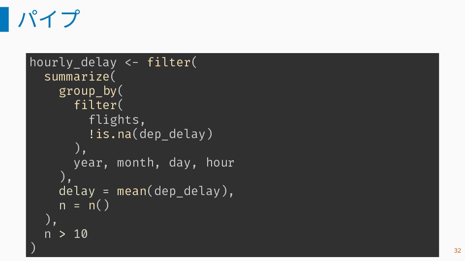
46. flights に airports を結合する location <- select(airports, dest = faa, name, lat, lon) flights %>% group_by(dest) %>% filter(!is.na(arr_delay)) %>% summarise(arr_delay = mean(arr_delay), n = n()) %>% arrange(desc(arr_delay)) %>% left_join(location) %>% select(-name) %>% slice(1:3) ## Joining, by = "dest" ## # A tibble: 3 x 5 ## dest arr_delay n lat lon ## <chr> <dbl> <int> <dbl> <dbl> ## 1 CAE 41.8 106 33.9 -81.1 ## 2 TUL 33.7 294 36.2 -95.9 ## 3 OKC 30.6 315 35.4 -97.6 46