OpenTalks.AI - Вадим Стрижов, Model generation for machine intelligence

Transcript

1. Model generation for machine intelligence Vadim Strijov Moscow Institute of Physics and Technology FRC CSC of the Russian Academy of Sciences 2018, February 7th 1 / 39
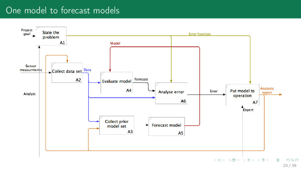
2. To start an applied project an expert and an analyst set 1. Project goal (the expected result of development) main purpose of research 2. Project application (how the project result will be applied) environment of measures and impacts 3. Historical data description (data formats and timing) algebraic structures of data 4. Quality criteria (how the project quality is measured) error function 5. Feasibility of the project (how to prove the project feasibility, list possible risks) error analysis How long the model lives after being put on operation? What replaces it after? 2 / 39
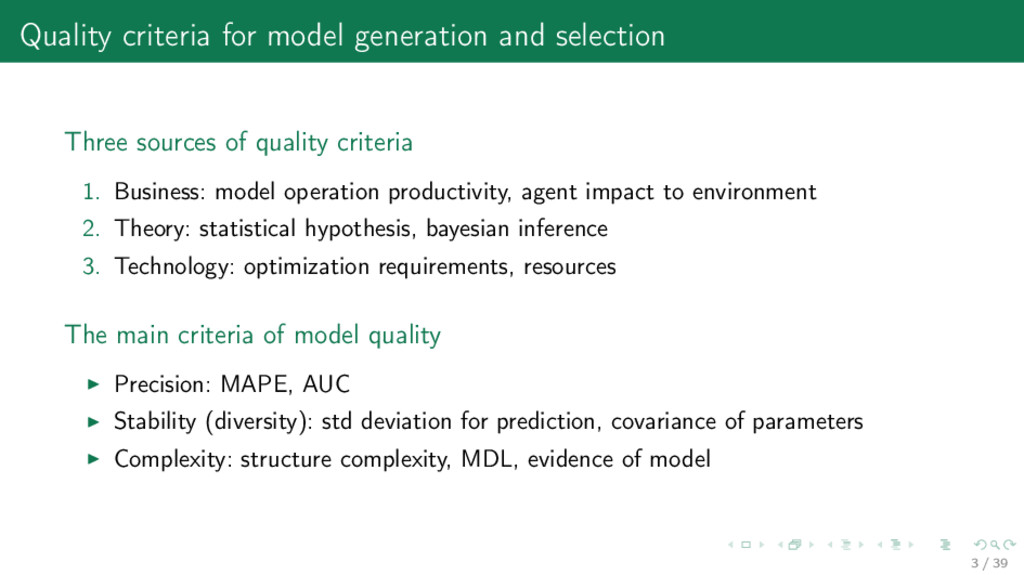
3. Quality criteria for model generation and selection Three sources of quality criteria 1. Business: model operation productivity, agent impact to environment 2. Theory: statistical hypothesis, bayesian inference 3. Technology: optimization requirements, resources The main criteria of model quality Precision: MAPE, AUC Stability (diversity): std deviation for prediction, covariance of parameters Complexity: structure complexity, MDL, evidence of model 3 / 39
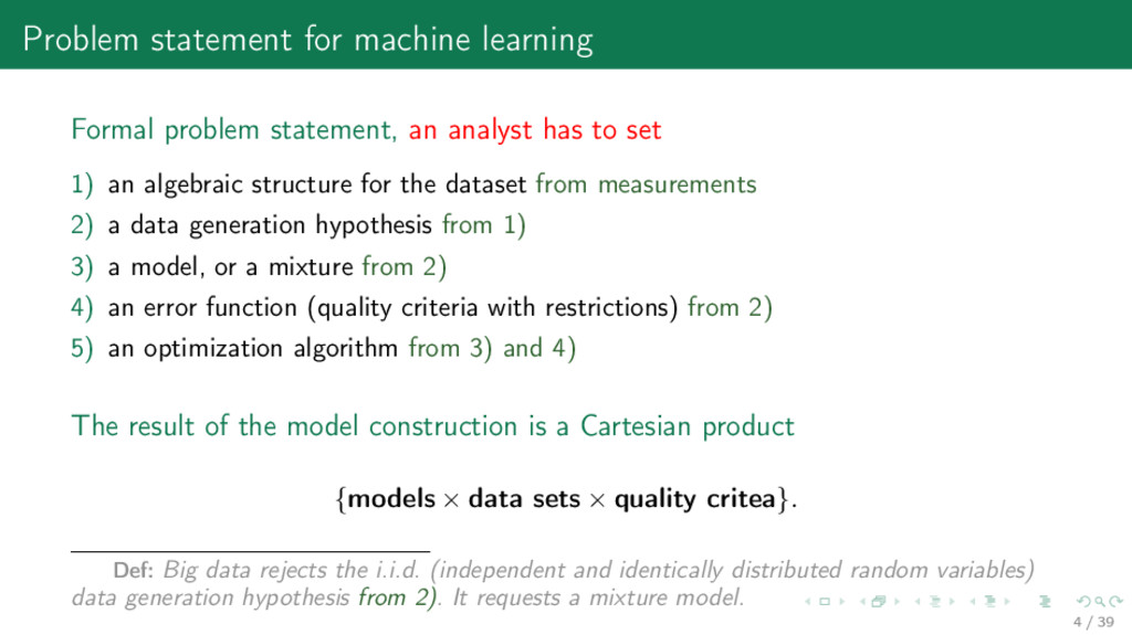
4. Problem statement for machine learning Formal problem statement, an analyst has to set 1) an algebraic structure for the dataset from measurements 2) a data generation hypothesis from 1) 3) a model, or a mixture from 2) 4) an error function (quality criteria with restrictions) from 2) 5) an optimization algorithm from 3) and 4) The result of the model construction is a Cartesian product {models × data sets × quality critea}. Def: Big data rejects the i.i.d. (independent and identically distributed random variables) data generation hypothesis from 2). It requests a mixture model. 4 / 39
5. Analyst creates a model for expert to put it to operation 5 / 39
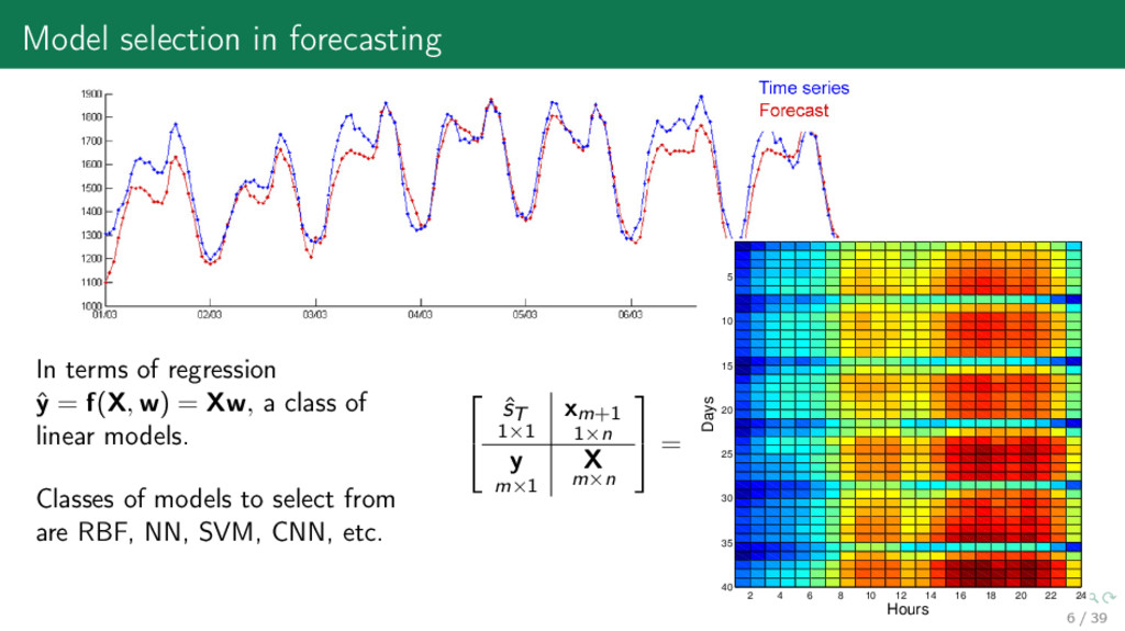
6. Model selection in forecasting In terms of regression ˆ y = f(X, w) = Xw, a class of linear models. Classes of models to select from are RBF, NN, SVM, CNN, etc.   ˆ sT 1×1 xm+1 1×n y m×1 X m×n   = 2 4 6 8 10 12 14 16 18 20 22 24 5 10 15 20 25 30 35 40 Hours Days 6 / 39
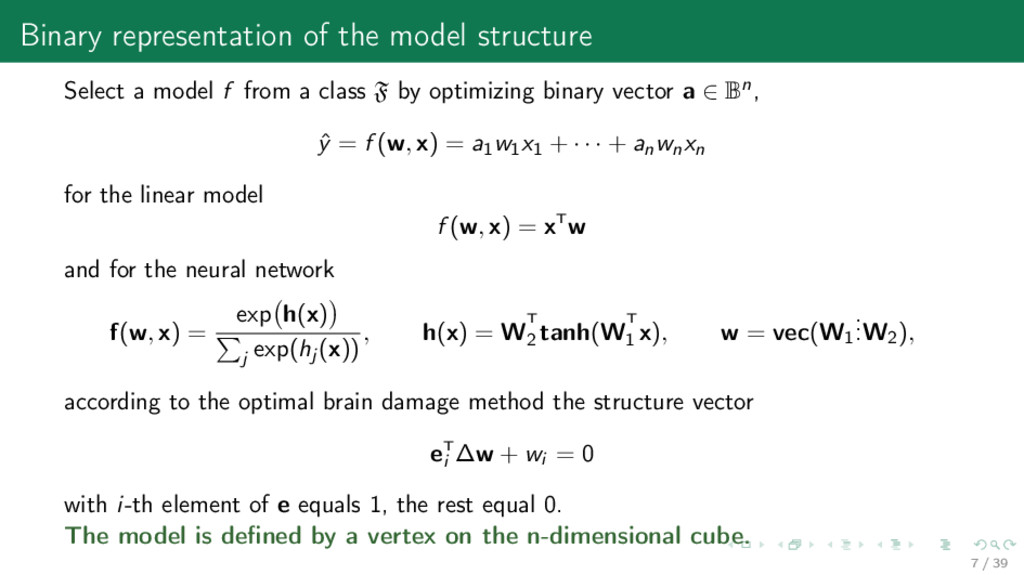
7. Binary representation of the model structure Select a model f from a class F by optimizing binary vector a ∈ Bn, ˆ y = f (w, x) = a1w1x1 + · · · + anwnxn for the linear model f (w, x) = xTw and for the neural network f(w, x) = exp h(x) j exp(hj (x)) , h(x) = WT 2 tanh(WT 1 x), w = vec(W1 . . .W2), according to the optimal brain damage method the structure vector eT i ∆w + wi = 0 with i-th element of e equals 1, the rest equal 0. The model is defined by a vertex on the n-dimensional cube. 7 / 39
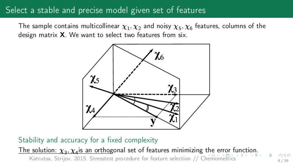
8. Select a stable and precise model given set of features The sample contains multicollinear χ1 , χ2 and noisy χ5 , χ6 features, columns of the design matrix X. We want to select two features from six. Stability and accuracy for a fixed complexity The solution: χ3 , χ4 is an orthogonal set of features minimizing the error function. Katrutsa, Strijov. 2015. Stresstest procedure for feature selection // Chemometrics 8 / 39
9. Model parameter values with regularization Vector-function f = f(w, X) = [f (w, x1), . . . , f (w, xm)]T ∈ Ym. 0 2 4 6 8 10 −15 −10 −5 0 5 10 15 20 25 30 Regularization, τ Parameters, w S(w) = f(w, X) − y 2 + γ2 w 2 0 2 4 6 8 −2 −1 0 1 2 3 Parameters sum, i |wi | Parameters, w S(w) = f(w, X) − y 2, T(w) τ 9 / 39
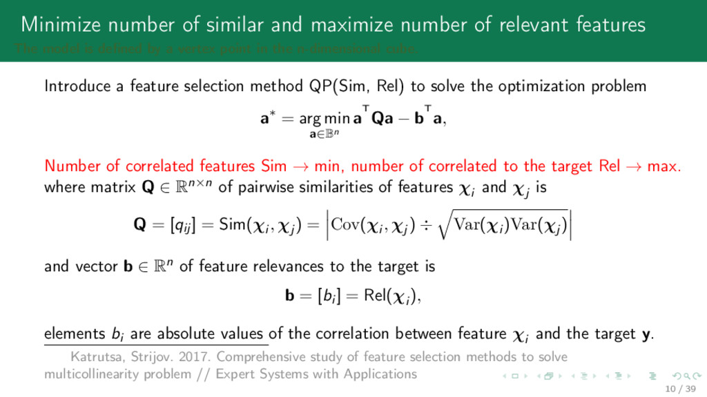
10. Minimize number of similar and maximize number of relevant features The model is defined by a vertex point in the n-dimensional cube. Introduce a feature selection method QP(Sim, Rel) to solve the optimization problem a∗ = arg min a∈Bn aT Qa − bT a, Number of correlated features Sim → min, number of correlated to the target Rel → max. where matrix Q ∈ Rn×n of pairwise similarities of features χi and χj is Q = [qij ] = Sim(χi , χj ) = Cov(χi , χj ) ÷ Var(χi )Var(χj ) and vector b ∈ Rn of feature relevances to the target is b = [bi ] = Rel(χi ), elements bi are absolute values of the correlation between feature χi and the target y. Katrutsa, Strijov. 2017. Comprehensive study of feature selection methods to solve multicollinearity problem // Expert Systems with Applications 10 / 39
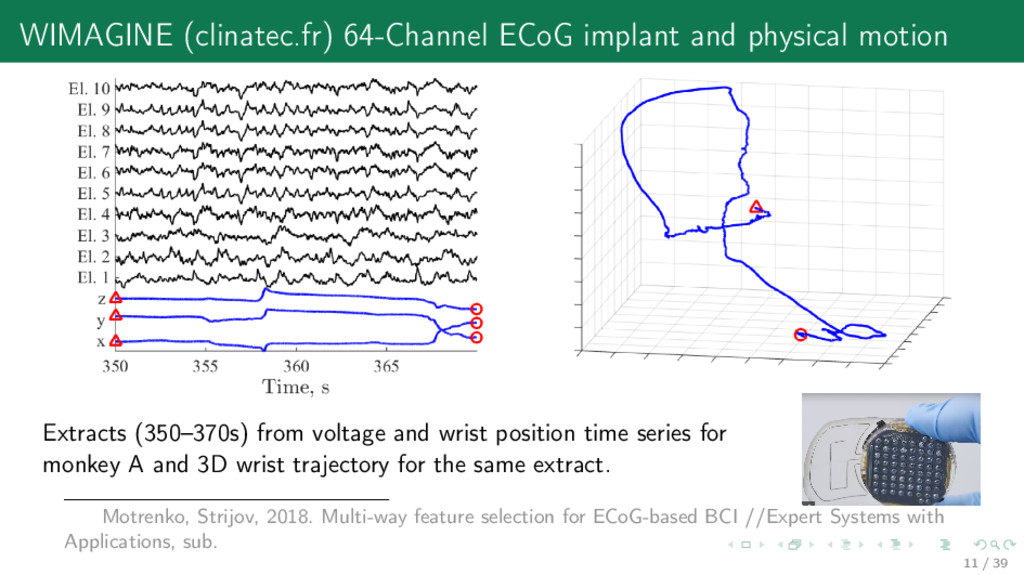
11. WIMAGINE (clinatec.fr) 64-Channel ECoG implant and physical motion Extracts (350–370s) from voltage and wrist position time series for monkey A and 3D wrist trajectory for the same extract. Motrenko, Strijov, 2018. Multi-way feature selection for ECoG-based BCI //Expert Systems with Applications, sub. 11 / 39
12. The wrist motion trajectory prediction with ECoG Segment of the forecasted time series. Linear regression, 50 best features according to multi-way QPFS (from 1000 highly-correlated features). 12 / 39
13. Empirical distribution of model parameters There given a sample {w1 , . . . , wK } of realizations of the m.r.v. w and an error function S(w|D, f). Analyze the set {sk = exp −S(wk |D, f) |k = 1, . . . , K}. 0 0.2 0.4 0 0.2 0.4 0.02 0.04 0.06 0.08 w2 w1 exp −S(w) 20 40 60 80 100 10 20 30 40 50 60 70 80 90 100 w1 w2 Kuznetsov, Tokmakova, Strijov. 2016. Analytic methods of structure parameter // Informatica 13 / 39
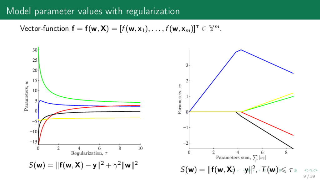
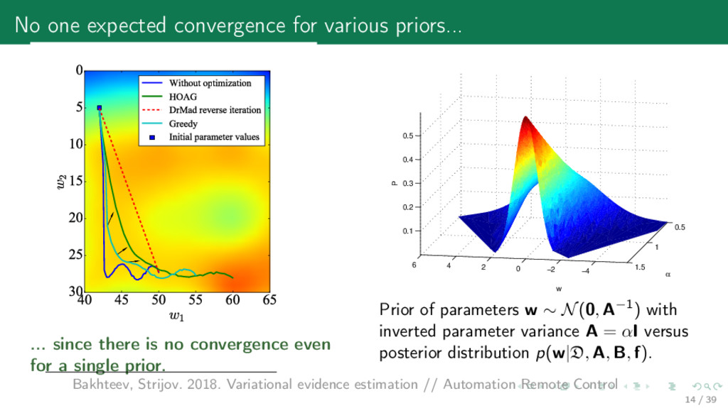
14. No one expected convergence for various priors... 40 45 50 55 60 65 w 1 0 5 10 15 20 25 30 w 2 Without optimization HOAG DrMad reverse iteration Greedy Initial parameter values ... since there is no convergence even for a single prior. −4 −2 0 2 4 6 0.5 1 1.5 0.1 0.2 0.3 0.4 0.5 α w P Prior of parameters w ∼ N(0, A−1) with inverted parameter variance A = αI versus posterior distribution p(w|D, A, B, f). Bakhteev, Strijov. 2018. Variational evidence estimation // Automation Remote Control 14 / 39
15. Forecasting quality does not change until almost all connections removed Model stability 0.0 0.1 0.2 0.3 0.4 0.5 0.0 0.2 0.4 0.6 0.8 1.0 Added noise variance Classification quality 60% removed Original model Redundancy of parameters 0 20 40 60 80 100 0.0 0.2 0.4 0.6 0.8 1.0 Classification quality Random Minimum Relevant Percentage of prunned parameters Def: Deep neural network is a model of exceeding complexity. It ignores the universal approximation theorem (George Cybenko 1989, Kurt Hornik 1991). 15 / 39
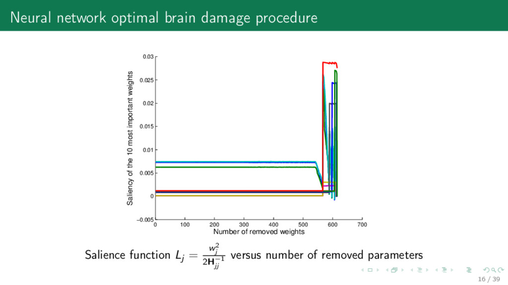
16. Neural network optimal brain damage procedure 0 100 200 300 400 500 600 700 −0.005 0 0.005 0.01 0.015 0.02 0.025 0.03 Number of removed weights Saliency of the 10 most important weights Salience function Lj = w2 j 2H−1 jj versus number of removed parameters 16 / 39
17. Consequent model generation Popova, Strijov. 2015. Selection of optimal physical activity classification model // Informatics and Applications 17 / 39
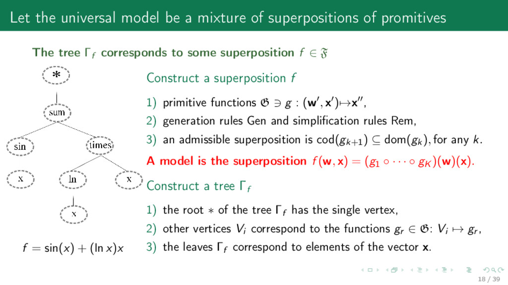
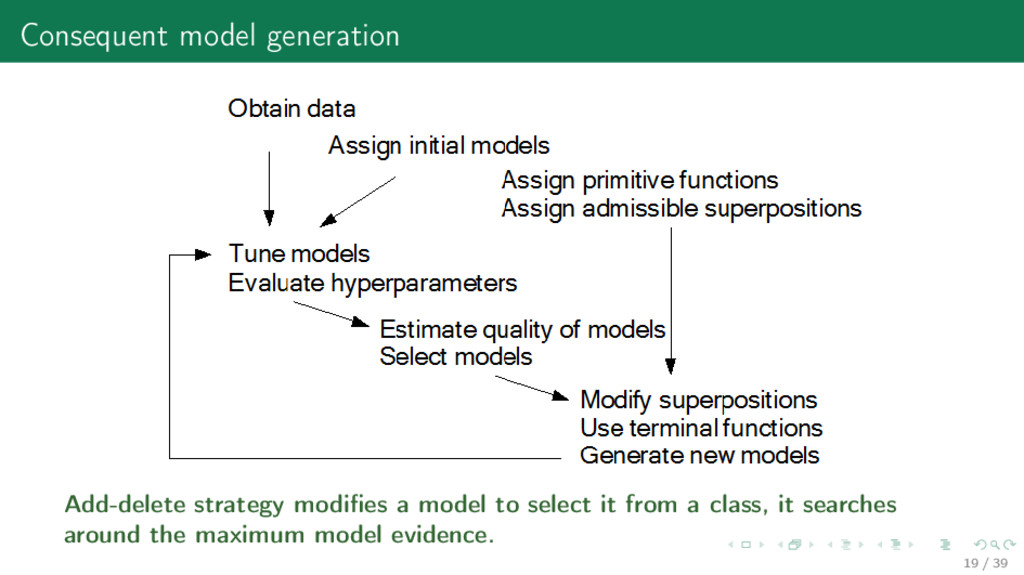
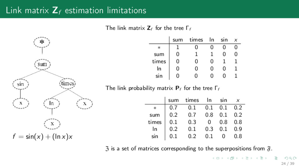
18. Let the universal model be a mixture of superpositions of promitives The tree Γf corresponds to some superposition f ∈ F f = sin(x) + (ln x)x Construct a superposition f 1) primitive functions G g : (w , x )→x , 2) generation rules Gen and simplification rules Rem, 3) an admissible superposition is cod(gk+1) ⊆ dom(gk), for any k. A model is the superposition f (w, x) = (g1 ◦ · · · ◦ gK )(w)(x). Construct a tree Γf 1) the root ∗ of the tree Γf has the single vertex, 2) other vertices Vi correspond to the functions gr ∈ G: Vi → gr , 3) the leaves Γf correspond to elements of the vector x. 18 / 39
19. Consequent model generation Add-delete strategy modifies a model to select it from a class, it searches around the maximum model evidence. 19 / 39
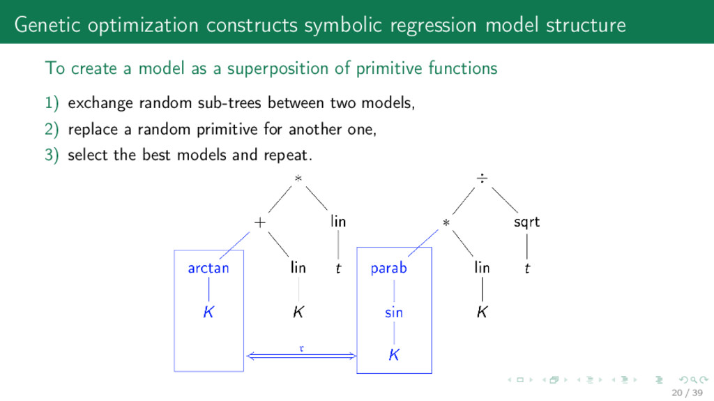
20. Genetic optimization constructs symbolic regression model structure To create a model as a superposition of primitive functions 1) exchange random sub-trees between two models, 2) replace a random primitive for another one, 3) select the best models and repeat. 20 / 39
21. Simple superposition has 14 parameters wersus 2-NN has 64 parameters Approximate the pressure in the combusting camera of a diesel engine 21 / 39
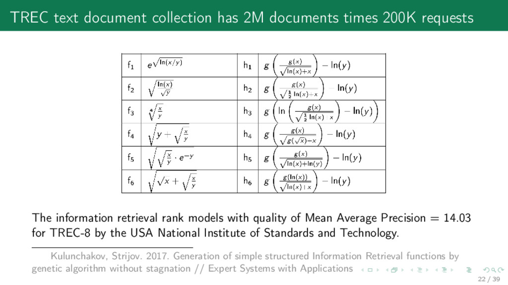
22. TREC text document collection has 2M documents times 200K requests The information retrieval rank models with quality of Mean Average Precision = 14.03 for TREC-8 by the USA National Institute of Standards and Technology. Kulunchakov, Strijov. 2017. Generation of simple structured Information Retrieval functions by genetic algorithm without stagnation // Expert Systems with Applications 22 / 39
23. One model to forecast models 23 / 39
24. Link matrix Zf estimation limitations f = sin(x) + (ln x)x The link matrix Zf for the tree Γf sum times ln sin x ∗ 1 0 0 0 0 sum 0 1 1 0 0 times 0 0 0 1 1 ln 0 0 0 0 1 sin 0 0 0 0 1 The link probability matrix Pf for the tree Γf sum times ln sin x ∗ 0.7 0.1 0.1 0.1 0.2 sum 0.2 0.7 0.8 0.1 0.2 times 0.1 0.3 0 0.8 0.8 ln 0.2 0.1 0.3 0.1 0.9 sin 0.1 0.2 0.1 0 0.8 Z is a set of matrices corresponding to the superpositions from F. 24 / 39
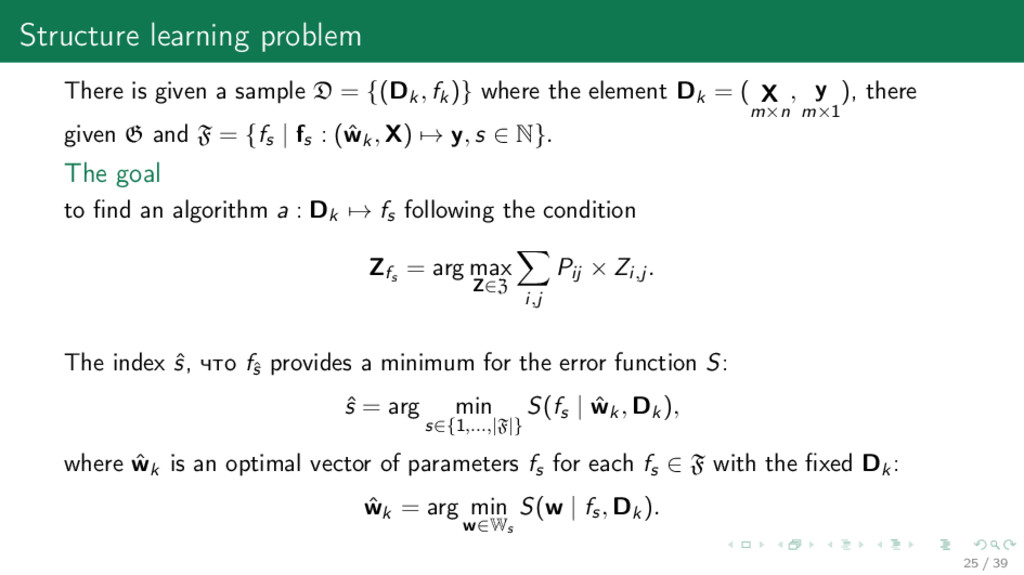
25. Structure learning problem There is given a sample D = {(Dk , fk)} where the element Dk = ( X m×n , y m×1 ), there given G and F = {fs | fs : (ˆ wk , X) → y, s ∈ N}. The goal to find an algorithm a : Dk → fs following the condition Zfs = arg max Z∈Z i,j Pij × Zi,j . The index ˆ s, что fˆ s provides a minimum for the error function S: ˆ s = arg min s∈{1,...,|F|} S(fs | ˆ wk , Dk), where ˆ wk is an optimal vector of parameters fs for each fs ∈ F with the fixed Dk: ˆ wk = arg min w∈Ws S(w | fs , Dk). 25 / 39
26. Complex action: workers construct a rack (Forecsys.ru, behavioral analysis) 26 / 39
27. Complex movement: the worker is drilling while standing x y z Acceleration time series [xt , yt , zt]T. 0 1 2 3 4 5 −0.5 0 0.5 1 1.5 2 Time t, s Acceleration, x,y, z Slow walking 0 1 2 3 4 −1 0 1 2 3 4 Time t, s Acceleration, x, y, z Jogging 27 / 39
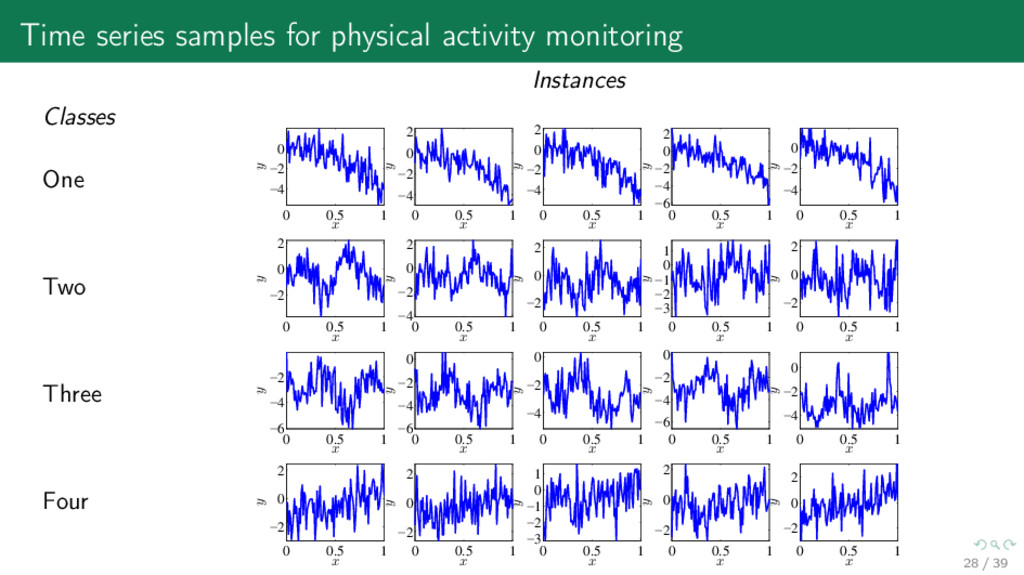
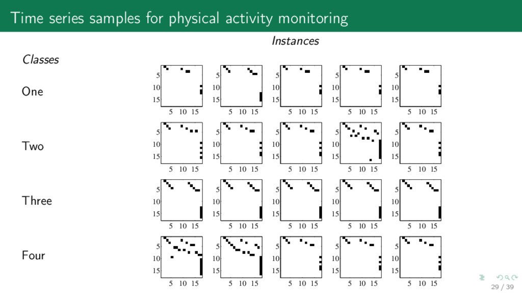
28. Time series samples for physical activity monitoring Classes One Two Three Four Instances 0 0.5 1 −4 −2 0 x y 0 0.5 1 −4 −2 0 2 x y 0 0.5 1 −4 −2 0 2 x y 0 0.5 1 −6 −4 −2 0 2 x y 0 0.5 1 −4 −2 0 x y 0 0.5 1 −2 0 2 x y 0 0.5 1 −4 −2 0 2 x y 0 0.5 1 −2 0 2 x y 0 0.5 1 −3 −2 −1 0 1 x y 0 0.5 1 −2 0 2 x y 0 0.5 1 −6 −4 −2 x y 0 0.5 1 −6 −4 −2 0 x y 0 0.5 1 −4 −2 0 x y 0 0.5 1 −6 −4 −2 0 x y 0 0.5 1 −4 −2 0 x y 0 0.5 1 −2 0 2 x y 0 0.5 1 −2 0 2 x y 0 0.5 1 −3 −2 −1 0 1 x y 0 0.5 1 −2 0 2 x y 0 0.5 1 −2 0 2 x y 28 / 39
29. Time series samples for physical activity monitoring Classes One Two Three Four Instances 5 10 15 5 10 15 5 10 15 5 10 15 5 10 15 5 10 15 5 10 15 5 10 15 5 10 15 5 10 15 5 10 15 5 10 15 5 10 15 5 10 15 5 10 15 5 10 15 5 10 15 5 10 15 5 10 15 5 10 15 5 10 15 5 10 15 5 10 15 5 10 15 5 10 15 5 10 15 5 10 15 5 10 15 5 10 15 5 10 15 5 10 15 5 10 15 5 10 15 5 10 15 5 10 15 5 10 15 5 10 15 5 10 15 5 10 15 5 10 15 29 / 39
30. The initial and the forecasted superposition 5 10 15 5 10 15 Ground truth 5 10 15 5 10 15 Forecasted probabilities 5 10 15 5 10 15 Forecasted superposition tree (model) 30 / 39
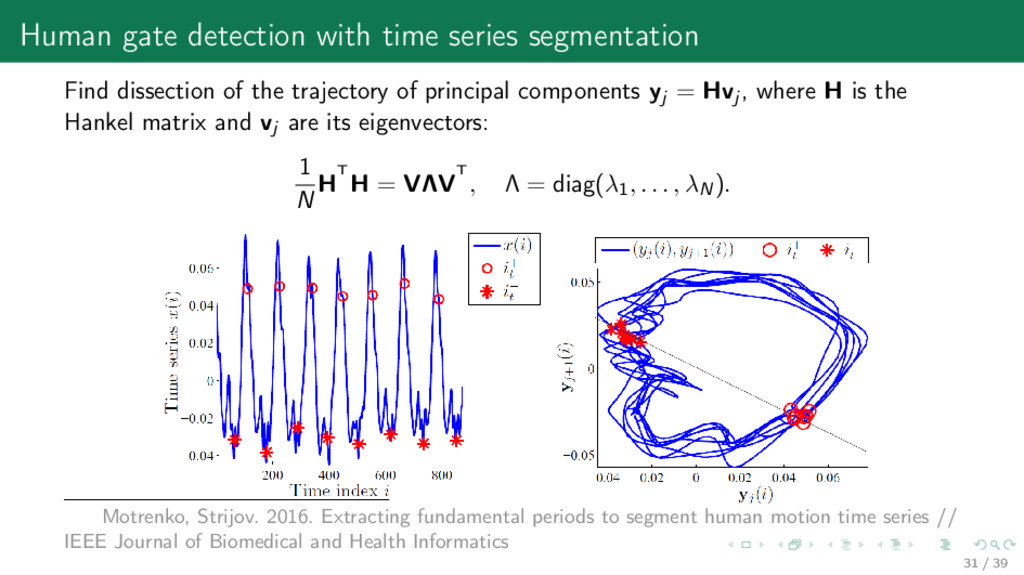
31. Human gate detection with time series segmentation Find dissection of the trajectory of principal components yj = Hvj , where H is the Hankel matrix and vj are its eigenvectors: 1 N HT H = VΛVT , Λ = diag(λ1 , . . . , λN). Motrenko, Strijov. 2016. Extracting fundamental periods to segment human motion time series // IEEE Journal of Biomedical and Health Informatics 31 / 39
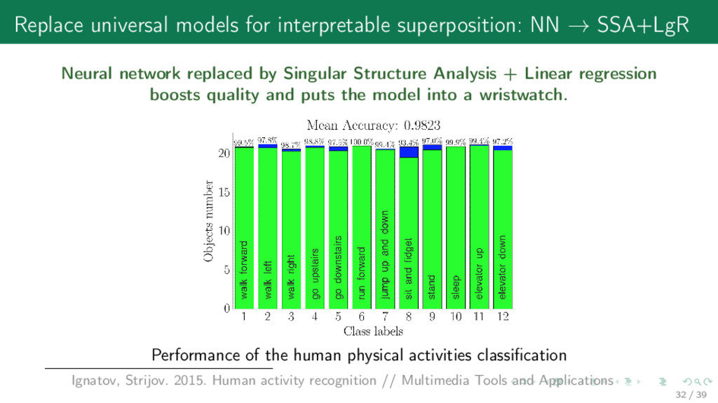
32. Replace universal models for interpretable superposition: NN → SSA+LgR Neural network replaced by Singular Structure Analysis + Linear regression boosts quality and puts the model into a wristwatch. Performance of the human physical activities classification Ignatov, Strijov. 2015. Human activity recognition // Multimedia Tools and Applications 32 / 39
33. Discover the iris by linear mixture (possible example) Replace a proprietary algorithm or CNN for mixture of linear models to drop the computational complexity. Example of interpretable modelling Chigrinsky. 2017. Modeling of the iris movement by optical flow//BS Thesis, adv. by Matveev 33 / 39
34. Put interpretable models to operation along with privilege learning models 34 / 39
35. Altae-Tran et al. 2016. Low data drug discovery with one-shot learning // arXiv 35 / 39
36. Altae-Tran et al. 2016. Low data drug discovery with one-shot learning // arXiv 36 / 39
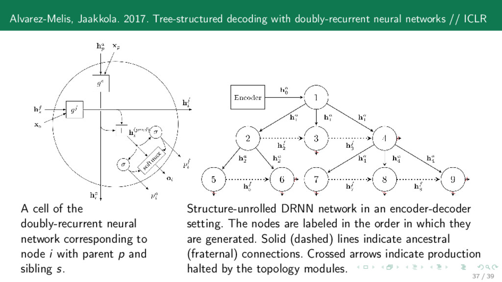
37. Alvarez-Melis, Jaakkola. 2017. Tree-structured decoding with doubly-recurrent neural networks // ICLR A cell of the doubly-recurrent neural network corresponding to node i with parent p and sibling s. Structure-unrolled DRNN network in an encoder-decoder setting. The nodes are labeled in the order in which they are generated. Solid (dashed) lines indicate ancestral (fraternal) connections. Crossed arrows indicate production halted by the topology modules. 37 / 39
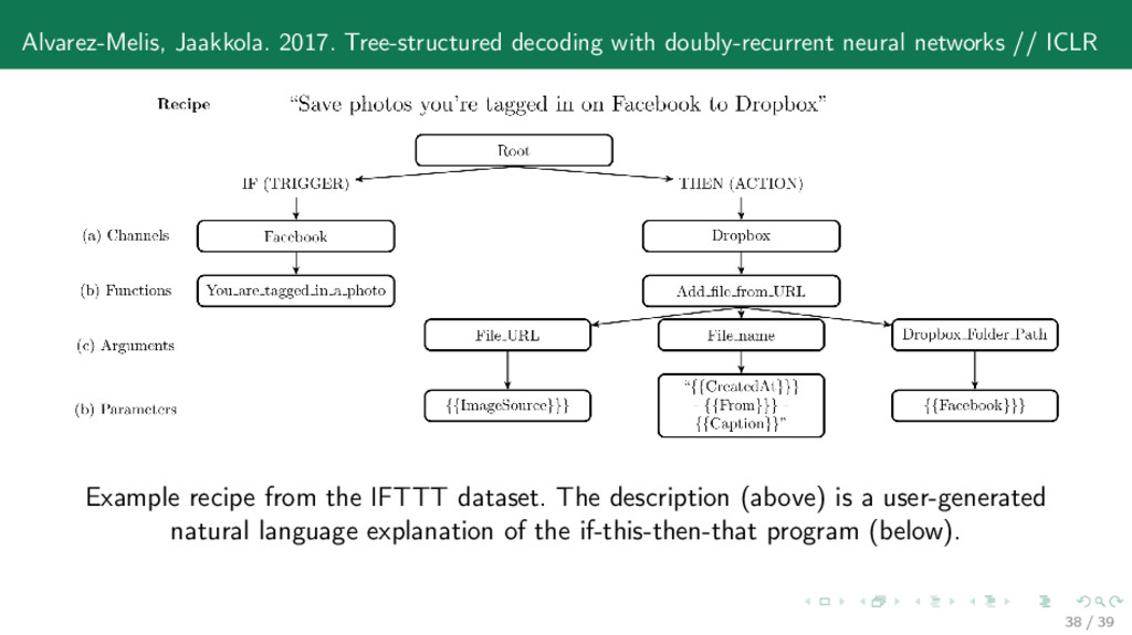
38. Alvarez-Melis, Jaakkola. 2017. Tree-structured decoding with doubly-recurrent neural networks // ICLR Example recipe from the IFTTT dataset. The description (above) is a user-generated natural language explanation of the if-this-then-that program (below). 38 / 39
39. List of the model generation principles 1. Binary/continuous/graph optimization of model structures 2. Neural networks forecast hyperparameters of neural networks (ref. NIPS 2017) 3. Networks forecast superpositions 4. Interpretable models replace neural network blocks 5. Company models boost quality of neighbor models by priviledge learning 39 / 39
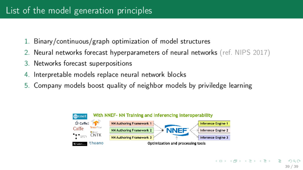
40. Our research challenges 1. Lay the foundations for the forecasting of model structures 2. Develop the theory of local modeling for signals of wearable devices 3. Deploy standards to exchange local and universal models 30+ projects starts 14.2.18. with 60 analysts, experts and MIPT students: 40 / 39