Accelerating MCMC with active subspaces

Talk at SIAM Conference on Uncertainty Quantification, April 2016

Transcript

1. Accelerating MCMC with active subspaces This material is based upon work supported by the U.S. Department of Energy Office of Science, Office of Advanced Scientific Computing Research, Applied Mathematics program under Award Number DE-SC-0011077. Thanks to: Youssef Marzouk Tiangang “TC” Cui Luis Tenorio PAUL CONSTANTINE Ben L. Fryrear Assistant Professor Applied Mathematics & Statistics Colorado School of Mines activesubspaces.org! @DrPaulynomial! SLIDES: DISCLAIMER: These slides are meant to complement the oral presentation. Use out of context at your own risk. Carson Kent Stanford Tan Bui-Thanh UT Austin
2. $27 VISIT THE SIAM BOOKSTORE! Coupon code: BKSL16
3. www.youtube.com/watch?v=mJvKzjT6lmY
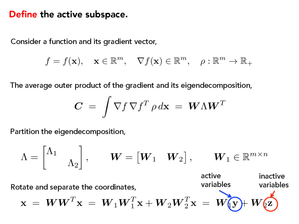
4. Define the active subspace. Consider a function and its gradient vector, The average outer product of the gradient and its eigendecomposition, Partition the eigendecomposition, Rotate and separate the coordinates, ⇤ =  ⇤1 ⇤2 , W = ⇥ W 1 W 2 ⇤ , W 1 2 Rm⇥n x = W W T x = W 1W T 1 x + W 2W T 2 x = W 1y + W 2z active variables inactive variables f = f( x ), x 2 Rm, rf( x ) 2 Rm, ⇢ : Rm ! R + C = Z rf rfT ⇢ d x = W ⇤W T
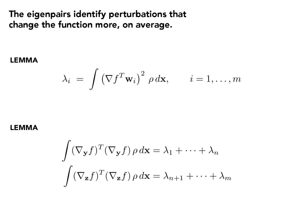
5. i = Z rfT wi 2 ⇢ d x , i = 1, . . . , m The eigenpairs identify perturbations that change the function more, on average. LEMMA LEMMA Z (ryf)T (ryf) ⇢ d x = 1 + · · · + n Z (rzf)T (rzf) ⇢ d x = n+1 + · · · + m
6. Discover the active subspace with Monte Carlo. Draw samples: Compute: and fj = f( xj) Approximate with Monte Carlo Equivalent to SVD of samples of the gradient Called an active subspace method in T. Russi’s 2010 Ph.D. thesis, Uncertainty Quantification with Experimental Data in Complex System Models xj ⇠ ⇢ C ⇡ 1 N N X j=1 rfj rfT j = ˆ W ˆ ⇤ ˆ W T 1 p N ⇥ rf1 · · · rfN ⇤ = ˆ W p ˆ ⇤ ˆ V T rfj = rf( xj)
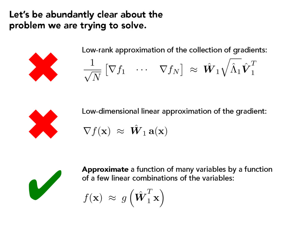
7. 1 p N ⇥ rf1 · · · rfN ⇤ ⇡ ˆ W 1 q ˆ ⇤1 ˆ V T 1 Low-rank approximation of the collection of gradients: Let’s be abundantly clear about the problem we are trying to solve. Low-dimensional linear approximation of the gradient: rf( x ) ⇡ ˆ W 1 a ( x ) f( x ) ⇡ g ⇣ ˆ W T 1 x ⌘ Approximate a function of many variables by a function of a few linear combinations of the variables: ✔ ✖ ✖
8. f( x ) ⇡ g ⇣ ˆ W T 1 x ⌘ How do you construct g? What is the approximation error? What is the effect of the approximate eigenvectors?
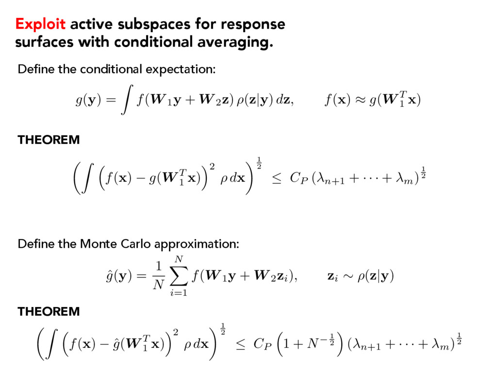
9. Define the conditional expectation: Define the Monte Carlo approximation: THEOREM g( y ) = Z f(W 1y + W 2z ) ⇢( z | y ) d z , f( x ) ⇡ g(W T 1 x ) ˆ g(y) = 1 N N X i=1 f(W 1y + W 2zi), zi ⇠ ⇢(z|y) Exploit active subspaces for response surfaces with conditional averaging. ✓Z ⇣ f( x ) g(W T 1 x ) ⌘2 ⇢ d x ◆1 2  CP ( n+1 + · · · + m)1 2 ✓Z ⇣ f( x ) ˆ g(W T 1 x ) ⌘2 ⇢ d x ◆1 2  CP ⇣ 1 + N 1 2 ⌘ ( n+1 + · · · + m)1 2 THEOREM
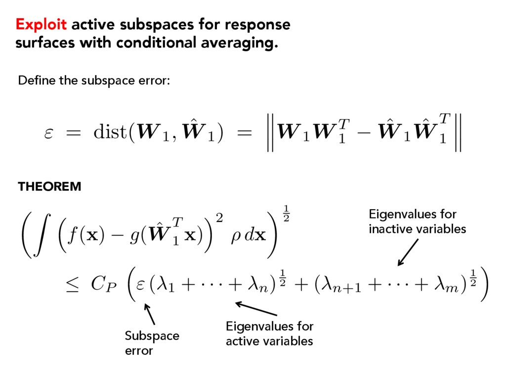
10. " = dist(W 1, ˆ W 1) = W 1W T 1 ˆ W 1 ˆ W T 1 ✓Z ⇣ f( x ) g( ˆ W T 1 x ) ⌘2 ⇢ d x ◆1 2  CP ⇣ " ( 1 + · · · + n)1 2 + ( n+1 + · · · + m)1 2 ⌘ Subspace error Eigenvalues for active variables Eigenvalues for inactive variables Define the subspace error: THEOREM Exploit active subspaces for response surfaces with conditional averaging.
11. 1.  Choose points in the domain of g. 2.  Estimate conditional average at each point. 3.  Construct the approximation* in n < m dimensions. ( * Don’t interpolate! )
12. INVERSION P(A|B) = P(B|A) P(A) P(B)
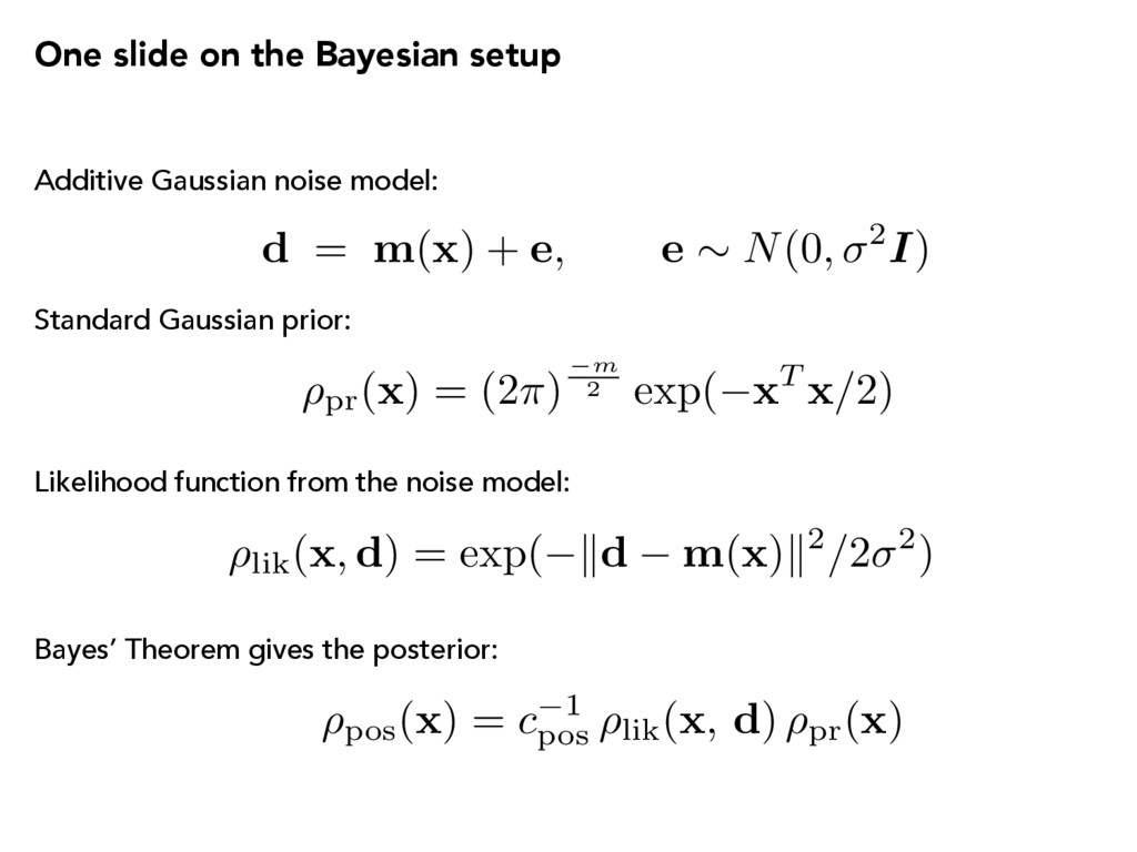
13. d = m ( x ) + e , e ⇠ N(0, 2I) ⇢lik(x , d) = exp( k d m(x) k2/ 2 2 ) ⇢ pos ( x ) = c 1 pos ⇢ lik ( x , d ) ⇢ pr ( x ) One slide on the Bayesian setup Additive Gaussian noise model: Standard Gaussian prior: Likelihood function from the noise model: Bayes’ Theorem gives the posterior: ⇢pr(x) = (2 ⇡ ) m 2 exp( x T x / 2)
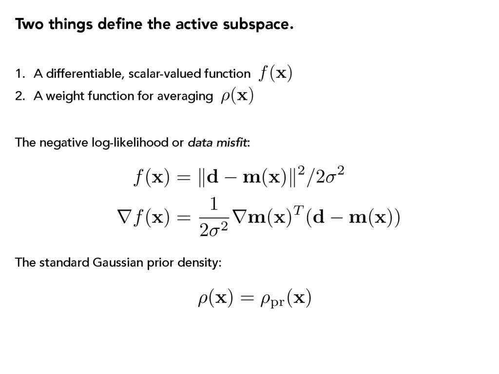
14. f( x ) = k d m ( x )k2/2 2 rf( x ) = 1 2 2 r m ( x )T ( d m ( x )) 1.  A differentiable, scalar-valued function 2.  A weight function for averaging Two things define the active subspace. ⇢( x ) f( x ) The negative log-likelihood or data misfit: The standard Gaussian prior density: ⇢( x ) = ⇢pr( x )
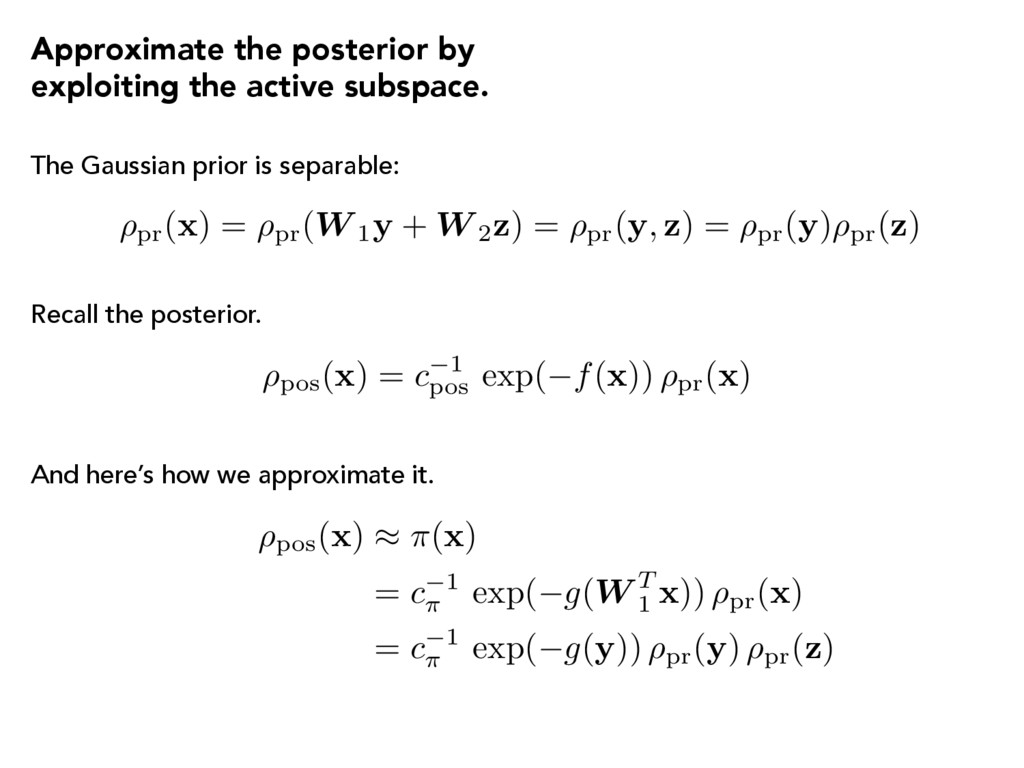
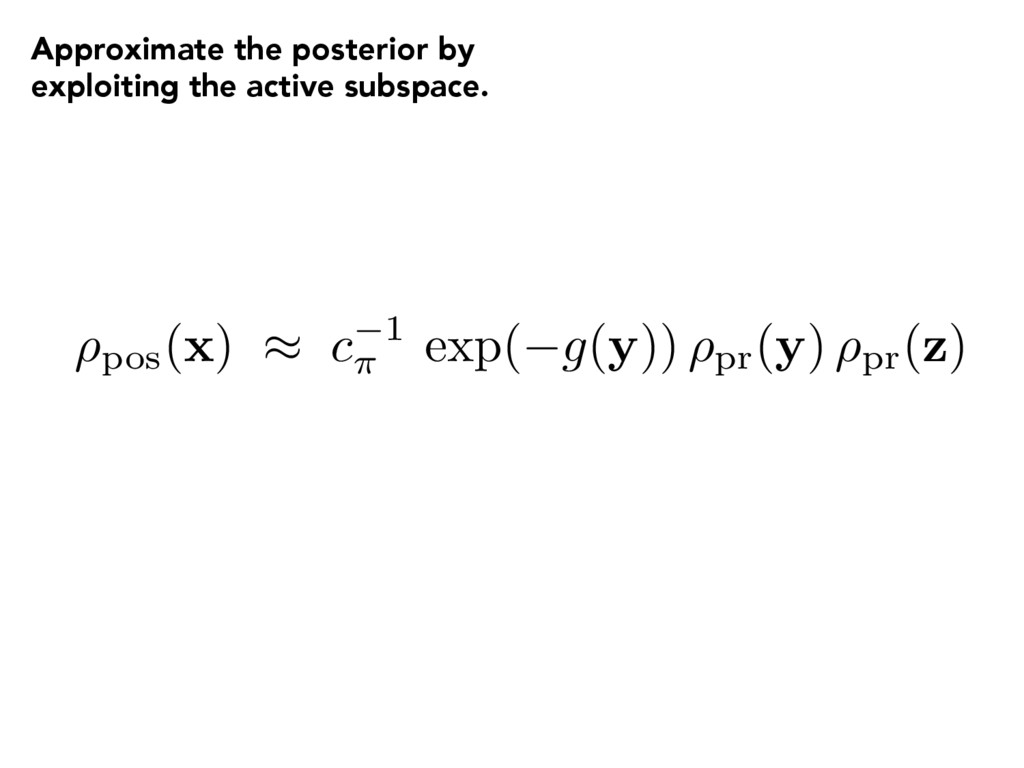
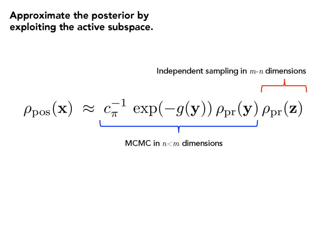
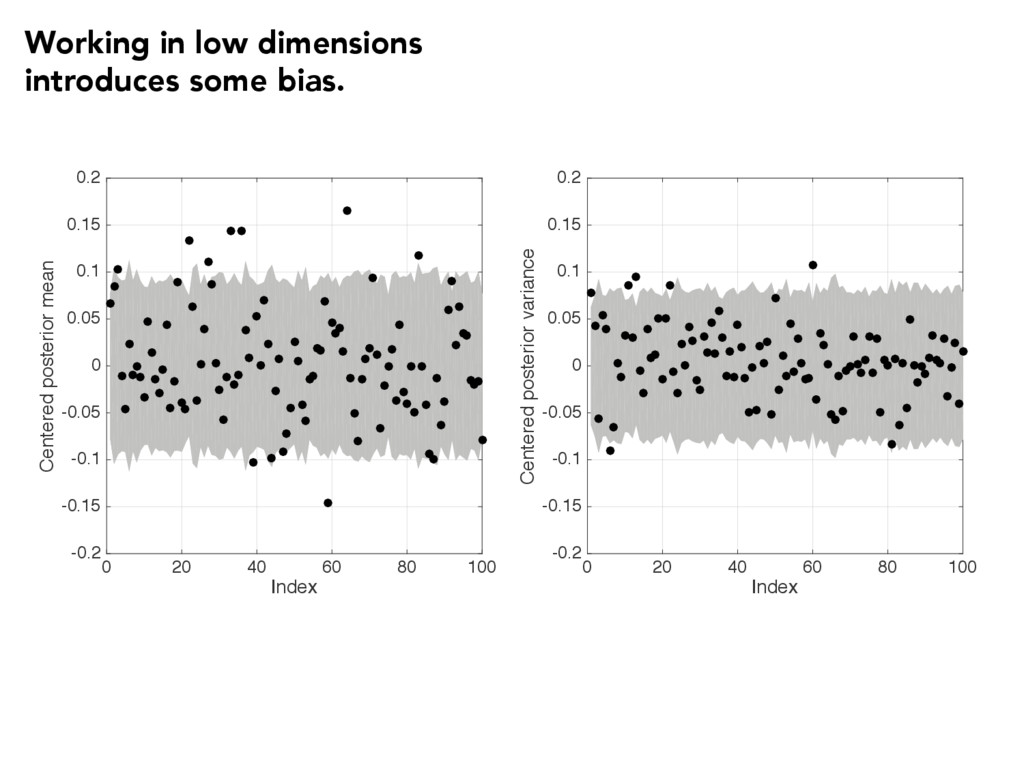
15. ⇢ pos(x) = c 1 pos exp( f (x)) ⇢ pr(x) ⇢ pos(x) ⇡ ⇡ (x) = c 1 ⇡ exp( g ( W T 1 x)) ⇢ pr(x) = c 1 ⇡ exp( g (y)) ⇢ pr(y) ⇢ pr(z) ⇢pr( x ) = ⇢pr(W 1y + W 2z ) = ⇢pr( y , z ) = ⇢pr( y )⇢pr( z ) Approximate the posterior by exploiting the active subspace. The Gaussian prior is separable: Recall the posterior. And here’s how we approximate it.
16. ⇢ pos(x) ⇡ c 1 ⇡ exp( g (y)) ⇢ pr(y) ⇢ pr(z) Approximate the posterior by exploiting the active subspace.
17. THEOREM Hellinger distance between posterior and approximation Eigenvalues for inactive variables The approximation error depends on the eigenvalues. ✓Z ⇣ ⇢ 1 2 pos ⇡ 1 2 ⌘ 2 d x ◆1 2  C ( n +1 + · · · + m)1 2
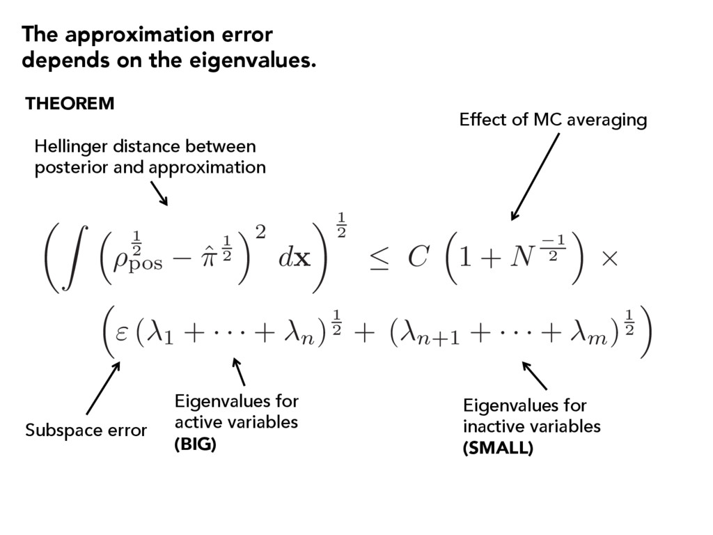
18. ✓Z ⇣ ⇢ 1 2 pos ˆ ⇡ 1 2 ⌘ 2 d x ◆1 2  C ⇣ 1 + N 1 2 ⌘ ⇥ ⇣ " ( 1 + · · · + n)1 2 + ( n +1 + · · · + m)1 2 ⌘ THEOREM Hellinger distance between posterior and approximation Eigenvalues for inactive variables (SMALL) The approximation error depends on the eigenvalues. Eigenvalues for active variables (BIG) Subspace error Effect of MC averaging
19. MCMC in n<m dimensions Independent sampling in m-n dimensions ⇢ pos(x) ⇡ c 1 ⇡ exp( g (y)) ⇢ pr(y) ⇢ pr(z) Approximate the posterior by exploiting the active subspace.
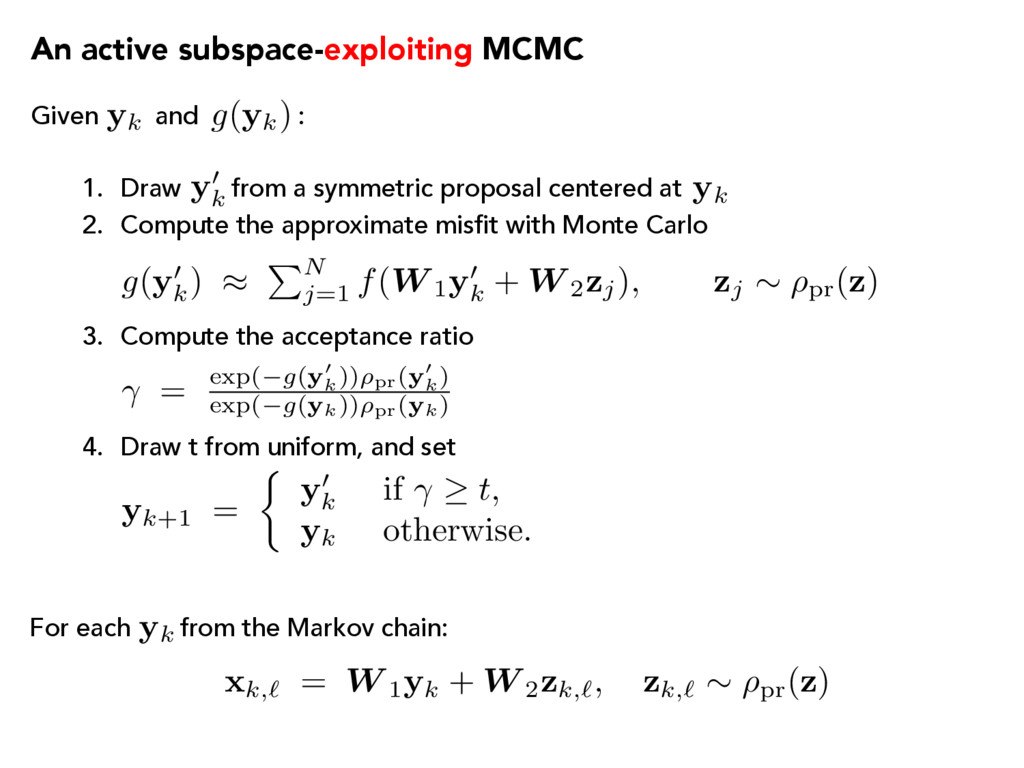
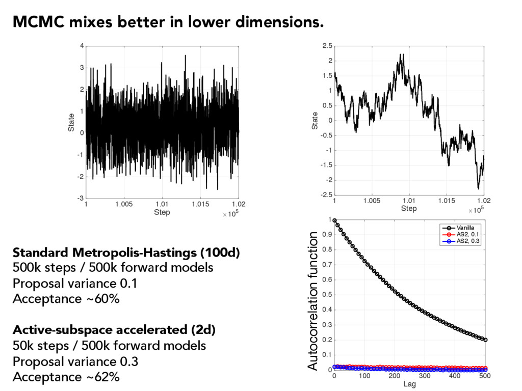
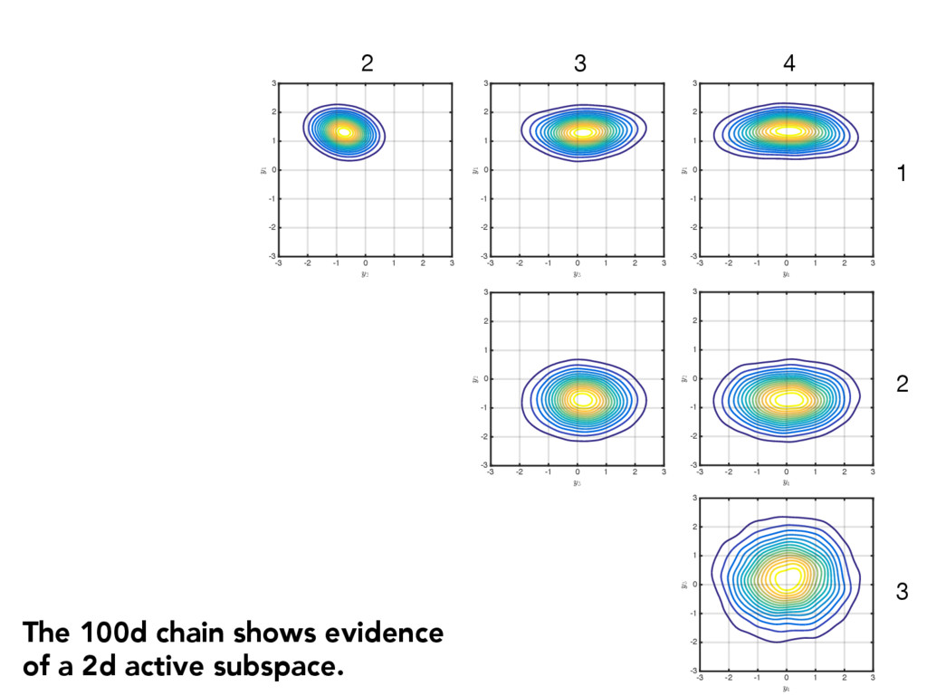
20. An active subspace-exploiting MCMC Given and : 1.  Draw from a symmetric proposal centered at 2.  Compute the approximate misfit with Monte Carlo 3.  Compute the acceptance ratio 4.  Draw t from uniform, and set yk y0 k yk g(y0 k ) ⇡ PN j=1 f(W 1y0 k + W 2zj), zj ⇠ ⇢pr(z) g(yk) = exp( g ( y0 k)) ⇢pr( y0 k) exp( g ( yk)) ⇢pr( yk) yk+1 = ⇢ y0 k if t , yk otherwise. yk For each from the Markov chain: xk,` = W 1yk + W 2zk,`, zk,` ⇠ ⇢pr( z )
21. [ Show them the MATLAB demo! ]
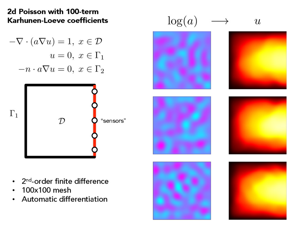
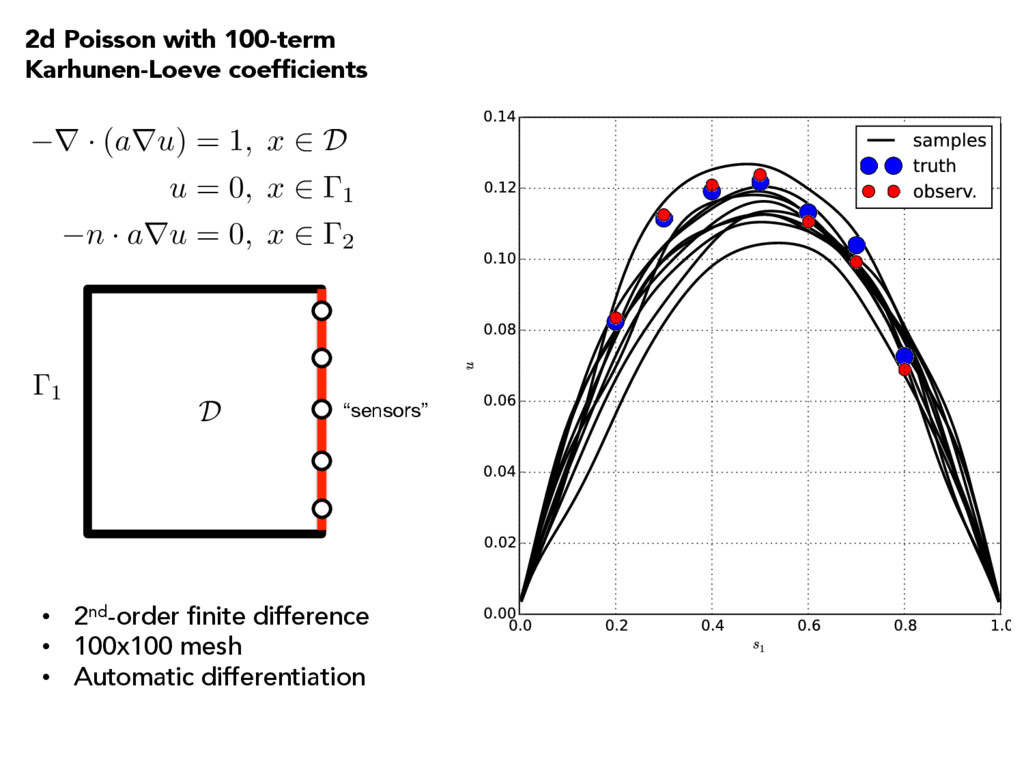
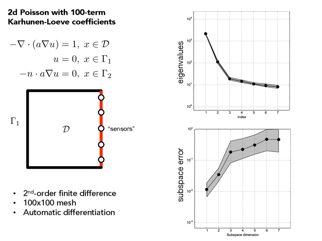
22. 2d Poisson with 100-term Karhunen-Loeve coefficients r · ( a r u ) = 1 , x 2 D u = 0 , x 2 1 n · a r u = 0 , x 2 2 1 D “sensors” log( a ) ! u •  2nd-order finite difference •  100x100 mesh •  Automatic differentiation
23. r · ( a r u ) = 1 , x 2 D u = 0 , x 2 1 n · a r u = 0 , x 2 2 1 D “sensors” •  2nd-order finite difference •  100x100 mesh •  Automatic differentiation 2d Poisson with 100-term Karhunen-Loeve coefficients
24. eigenvalues subspace error r · ( a r u ) = 1 , x 2 D u = 0 , x 2 1 n · a r u = 0 , x 2 2 1 D “sensors” •  2nd-order finite difference •  100x100 mesh •  Automatic differentiation 2d Poisson with 100-term Karhunen-Loeve coefficients
25. 1 1.005 1.01 1.015 1.02 Step #105 -2.5 -2 -1.5 -1 -0.5 0 0.5 1 1.5 2 2.5 State 1 1.005 1.01 1.015 1.02 Step #105 -3 -2 -1 0 1 2 3 4 State 0 100 200 300 400 500 Lag 0 0.1 0.2 0.3 0.4 0.5 0.6 0.7 0.8 0.9 1 Autocorrelation Vanilla AS2, 0.1 AS2, 0.3 Autocorrelation function MCMC mixes better in lower dimensions. Standard Metropolis-Hastings (100d) 500k steps / 500k forward models Proposal variance 0.1 Acceptance ~60% Active-subspace accelerated (2d) 50k steps / 500k forward models Proposal variance 0.3 Acceptance ~62%
26. Working in low dimensions introduces some bias. 0 20 40 60 80 100 Index -0.2 -0.15 -0.1 -0.05 0 0.05 0.1 0.15 0.2 Centered posterior mean 0 20 40 60 80 100 Index -0.2 -0.15 -0.1 -0.05 0 0.05 0.1 0.15 0.2 Centered posterior variance
27. -3 -2 -1 0 1 2 3 y2 -3 -2 -1 0 1 2 3 y1 -3 -2 -1 0 1 2 3 y3 -3 -2 -1 0 1 2 3 y1 -3 -2 -1 0 1 2 3 y4 -3 -2 -1 0 1 2 3 y1 -3 -2 -1 0 1 2 3 y3 -3 -2 -1 0 1 2 3 y2 -3 -2 -1 0 1 2 3 y4 -3 -2 -1 0 1 2 3 y2 -3 -2 -1 0 1 2 3 y4 -3 -2 -1 0 1 2 3 y3 1 2 3 2 3 4 The 100d chain shows evidence of a 2d active subspace.
28. •  How do active subspaces relate to [insert method]? •  How does this work with a linear forward model? •  What kinds of models does this work on? PAUL CONSTANTINE Ben L. Fryrear Assistant Professor Colorado School of Mines activesubspaces.org! @DrPaulynomial! QUESTIONS?