Who give you th epsilon? J. V. Grabiner

Transcript

1. Who Gave You the Epsilon? Cauchy and the Origins of Rigorous Calculus Judith V. Grabiner, 424 West 7th Street, Claremont, California 91711 The American Mathematical Monthly, March 1983, Volume 90, Number 3, pp. 185–194. Student: The car has a speed of 50 miles an hour. What does that mean? Teacher: Given any there exists a such that if then Student: How in the world did anybody ever think of such an answer? Perhaps this exchange will remind us that the rigorous basis for the calculus is not at all intuitive—in fact, quite the contrary. The calculus is a subject dealing with speeds and distances, with tangents and areas—not inequalities. When Newton and Leibniz invented the calculus in the late seventeenth century, they did not use delta- epsilon proofs. It took a hundred and fifty years to develop them. This means that it was probably very hard, and it is no wonder that a modern student finds the rigorous basis of the calculus difficult. How, then, did the calculus get a rigorous basis in terms of the algebra of inequalities? Delta-epsilon proofs are first found in the works of Augustin-Louis Cauchy (1789–1867). This is not always recognized, since Cauchy gave a purely verbal definition of limit, which at first glance does not resemble modern definitions: “When the successively attributed values of the same variable indefinitely approach a fixed value, so that finally they differ from it by as little as desired, the last is called the limit of all the others’’ [1]. Cauchy also gave a purely verbal definition of the derivative of as the limit, when it exists, of the quotient of differences when h goes to zero, a statement much like those that had already been made by Newton, Leibniz, d’Alembert, Maclaurin, and Euler. But what is significant is that Cauchy translated such verbal statements into the precise language of inequalities when he needed them in his proofs. For instance, for the derivative [2]: (1) Let be two very small numbers; the first is chosen so that for all numerical [i.e., absolute] values of h less than and for any value of x included [in the interval of definition], the ratio will always be greater than and less than This one example will be enough to indicate how Cauchy did the calculus, because the question to be answered in the present paper is not, “how is a rigorous delta-epsilon proof constructed?’’As Cauchy’s intellectual heirs we all know this. The central question is, how and why was Cauchy able to put the calculus on a rigorous basis, when his predecessors were not? The answers to this historical question cannot be found by reflecting on the logical relations between the concepts, but by looking in detail at the past and seeing how the existing state of affairs in fact developed from that past. Thus we will examine the mathematical situation in the seventeenth and eighteenth centuries—the background against which we can appreciate Cauchy’s innovation. We will describe the powerful techniques of the calculus of this earlier period and the fЈ͑x͒ ϩ ␧. fЈ͑x͒ Ϫ ␧ ͑ f ͑x ϩ h͒ Ϫ f ͑x͒͒͞h ␦, ␦, ␧ ͑ f ͑x ϩ h͒ Ϫ f ͑x͒͒͞h f ͑x͒ Խs2 Ϫ s1 t2 Ϫ t1 Ϫ 50 Խ < ␧. Խt2 Ϫ t1 Խ < ␦, ␦ ␧ > 0,
2. relatively unimpressive views put forth to justify them. We will then discuss how a sense of urgency about rigorizing analysis gradually developed in the eighteenth century. Most important, we will explain the development of the mathematical techniques necessary for the new rigor from the work of men like Euler, d’Alembert, Poisson, and especially Lagrange. Finally, we will show how these mathematical results, though often developed for purposes far removed from establishing foundations for the calculus, were used by Cauchy in constructing his new rigorous analysis. The Practice of Analysis: From Newton to Euler. In the late seventeenth century, Newton and Leibniz, almost simultaneously, independently invented the calculus. This invention involved three things. First, they invented the general concepts of differential quotient and integral (these are Leibniz’s terms; Newton called the concepts “fluxion’’ and “fluent’’). Second, they devised a notation for these concepts which made the calculus an algorithm: the methods not only worked, but were easy to use. Their notations had great heuristic power, and we still use Leibniz’s and and Newton’s today. Third, both men realized that the basic processes of finding tangents and areas, that is, differentiating and integrating, are mutually inverse—what we now call the Fundamental Theorem of Calculus. Once the calculus had been invented, mathematicians possessed an extremely powerful set of methods for solving problems in geometry, in physics, and in pure analysis. But what was the nature of the basic concepts? For Leibniz, the differential quotient was a ratio of infinitesimal differences, and the integral was a sum of infinitesimals. For Newton, the derivative, or fluxion, was described as a rate of change; the integral, or fluent, was its inverse. In fact, throughout the eighteenth century, the integral was generally thought of as the inverse of the differential. One might imagine asking Leibniz exactly what an infinitesimal was, or Newton what a rate of change might be. Newton’s answer, the best of the eighteenth century, is instructive. Consider a ratio of finite quantities (in modern notation, as h goes to zero). The ratio eventually becomes what Newton called an “ultimate ratio.’’ Ultimate ratios are “limits to which the ratios of quantities decreasing without limit do always converge, and to which they approach nearer than by any given difference, but never go beyond, nor ever reach until the quantities vanish’’ [3]. Except for “reaching’’ the limit when the quantities vanish, we can translate Newton’s words into our algebraic language. Newton himself, however, did not do this, nor did most of his followers in the eighteenth century. Moreover, “never go beyond’’ does not allow a variable to oscillate about its limit. Thus, though Newton’s is an intuitively pleasing picture, as it stands it was not and could not be used for proofs about limits. The definition sounds good, but it was not understood or applied in algebraic terms. But most eighteenth-century mathematicians would object, “Why worry about foundations?’’ In the eighteenth century, the calculus, intuitively understood and algorithmically executed, was applied to a wide range of problems. For instance, the partial differential equation for vibrating strings was solved; the equations of motion for the solar system were solved; the Laplace transform and the calculus of variations and the gamma function were invented and applied; all of mechanics was worked out in the language of the calculus. These were great achievements on the part of eighteenth- ͑ f ͑x ϩ h͒ Ϫ f ͑x͒͒͞h x . , ͐y dx, dy͞dx 2
3. century mathematicians. Who would be greatly concerned about foundations when such important problems could be successfully treated by the calculus? Results were what counted. This point will be better appreciated by looking at an example which illustrates both the “uncritical’’ approach to concepts of the eighteenth century and the immense power of eighteenth-century techniques, from the work of the great master of such techniques: Leonhard Euler. The problem is to find the sum of the series It clearly has a finite sum since it is bounded above by the series whose sum was known to be 2; Johann Bernoulli had found this sum by treating as the difference between the series and the series and observing that this difference telescopes [4]. Euler’s summation of makes use of a lemma from the theory of equations: given a polynomial equation whose constant term is one, the coefficient of the linear term is the product of the reciprocals of the roots with the signs changed. This result was both discovered and demonstrated by considering the equation having roots a and b. Multiplying and then dividing out ab, we obtain the result is now obvious, as is the extension to equations of higher degree. Euler’s solution then considers the equation sin Expanding this as an infinite series, Euler obtained Dividing by x yields Finally, substituting produces But Euler thought that power series could be manipulated just like polynomials. Thus, we now have a polynomial equation in u, whose constant term is one. Applying the lemma to it, the coefficient of the linear term with the sign changed is The roots of the equation in u are the roots of with the substitution namely . . . . Thus the lemma implies 1͞6 ϭ 1͞␲2 ϩ 1͑͞4␲2͒ϩ1͑͞9␲2͒ ϩ . . . . 9␲2, 4␲2, ␲2, u ϭ x2, sin x ϭ 0 1͞3! ϭ 1͞6. 1 Ϫ u͞3! ϩ u2͞5! Ϫ . . . ϭ 0. x2 ϭ u 1 Ϫ x2͞3! ϩ x 4͞5! Ϫ . . . ϭ 0. x Ϫ x3͞3! ϩ x5͞5! Ϫ . . . ϭ 0. x ϭ 0. ͑1͞ab͒x2 Ϫ ͑1͞a ϩ 1͞b͒x ϩ 1 ϭ 0; ͑x Ϫ a͒͑x Ϫ b͒ ϭ 0, ͚ ϱ kϭ1 1͞k2 1͞2 ϩ 1͞3 ϩ 1͞4 ϩ . . ., 1͞1 ϩ 1͞2 ϩ 1͞3 ϩ . . . 1͑͞1 и 2͒ ϩ 1͑͞2 и 3͒ ϩ 1͑͞3 и 4͒ ϩ . . . 1 ϩ 1͑͞1 и 2͒ ϩ 1͑͞2 и 3͒ ϩ 1͑͞3 и 4͒ ϩ . . . ϩ 1͓͑͞k Ϫ 1͒ и k͔ ϩ . . ., 1͞1 ϩ 1͞4 ϩ 1͞9 ϩ . . . ϩ 1͞k2 ϩ . . .. 3
4. Multiplying by yields the sum of the original series [5]: Though it is easy to criticize eighteenth-century arguments like this for their lack of rigor, it is also unfair. Foundations, precise specifications of the conditions under which such manipulations with infinites or infinitesimals were admissible, were not very important to men like Euler, because without such specifications they made important new discoveries, whose results in cases like this could readily be verified. When the foundations of the calculus were discussed in the eighteenth century, they were treated as secondary. Discussions of foundations appeared in the introductions to books, in popularizations, and in philosophical writings, and were not—as they are now and have been since Cauchy’s time—the subject of articles in research-oriented journals. Thus, where we once had one question to answer, we now have two. The first remains, where do Cauchy’s rigorous techniques come from? Second, one must now ask, why rigorize the calculus in the first place? If few mathematicians were very interested in foundations in the eighteenth century [6], then when, and why, were attitudes changed? Of course, to establish rigor, it is necessary—though not sufficient—to think rigor is significant. But more important, to establish rigor, it is necessary (though also not sufficient) to have a set of techniques in existence which are suitable for that purpose. In particular, if the calculus is to be made rigorous by being reduced to the algebra of inequalities, one must have both the algebra of inequalities, and facts about the concepts of the calculus that can be expressed in terms of the algebra of inequalities. In the early nineteenth century, three conditions held for the first time: Rigor was considered important; there was a well-developed algebra of inequalities; and, certain properties were known about the basic concepts of analysis—limits, convergence, continuity, derivatives, integrals—properties which could be expressed in the language of inequalities if desired. Cauchy, followed by Riemann and Weierstrass, gave the calculus a rigorous basis, using the already-existing algebra of inequalities, and built a logically-connected structure of theorems about the concepts of the calculus. It is our task to explain how these three conditions—the developed algebra of inequalities, the importance of rigor, the appropriate properties of the concepts of the calculus—came to be. The Algebra of Inequalities. Today, the algebra of inequalities is studied in calculus courses because of its use as a basis for the calculus, but why should it have been studied in the eighteenth century when this application was unknown? In the eighteenth century, inequalities were important in the study of a major class of results: approximations. For example, consider an equation such as for not an integer. Usually a cannot be found exactly, but it can be approximated by an infinite series. In general, given some number n of terms of such an approximating series, eighteenth-century mathematicians sought to compute an upper upper bound on the error in the approximation—that is, the difference between the sum of the series and the nth partial sum. This computation was a problem in the algebra of inequalities. Jean d’Alembert solved it for the important case of the binomial series; given the number of terms of the series n, and assuming implicitly that the series converges to its sum, he could find the bounds on the error—that is, on the remainder of the series after the nth ␮ ͑x ϩ 1͒␮ ϭ a, 1͞1 ϩ 1͞4 ϩ 1͞9 ϩ . . . ϩ 1͞k2 ϩ . . . ϭ ␲2͞6. ␲2 4
5. term—by bounding the series above and below with convergent geometric progressions [7]. Similarly, Joseph-Louis Lagrange invented a new approximation method using continued fractions and, by extremely intricate inequality-calculations, gave necessary and sufficient conditions for a given iteration of the approximation to be closer to the result than the previous iteration [8]. Lagrange also derived the Lagrange remainder of the Taylor series [9], using an inequality which bounded the remainder above and below by the maximum and minimum values of the nth derivative and then applying the intermediate-value theorem for continuous functions. Thus through such eighteenth- century work [10], there was by the end of the eighteenth century a developed algebra of inequalities, and people used to working with it. Given an n, these people are used to finding an error—that is, an epsilon. Changing Attitudes toward Rigor. Mathematicians were much more interested in finding rigorous foundations for the calculus in 1800 than they had been a hundred years before. There are many reasons for this: no one enough by itself, but apparently sufficient when acting together. Of course one might think that eighteenth-century mathematicians were always making errors because of the lack of an explicitly- formulated rigorous foundation. But this did not occur. They were usually right, and for two reasons. One is that if one deals with real variables, functions of one variable, series which are power series, and functions arising from physical problems, errors will not occur too often. A second reason is that mathematicians like Euler and Laplace had a deep insight into the basic properties of the concepts of the calculus, and were able to choose fruitful methods and evade pitfalls. The only “error’’ they committed was to use methods that shocked mathematicians of later ages who had grown up with the rigor of the nineteenth century. What then were the reasons for the deepened interest in rigor? One set of reasons was philosophical. In 1734, the British philosopher Bishop Berkeley had attacked the calculus on the ground that it was not rigorous. In The Analyst, or a Discourse Addressed to an Infidel Mathematician, he said that mathematicians had no business attacking the unreasonableness of religion, given the way they themselves reasoned. He ridiculed fluxions— “velocities of evanescent increments’’—calling the evanescent increments “ghosts of departed quantities’’ [11]. Even more to the point, he correctly criticized a number of specific arguments from the writings of his mathematical contemporaries. For instance, he attacked the process of finding the fluxion (our derivative) by reviewing the steps of the process: if we consider taking the ratio of the differences then simplifying to then letting h vanish, we obtain But is h zero? If it is, we cannot meaningfully divide by it; if it is not zero, we have no right to throw it away. As Berkeley put it, the quantity we have called h “might have signified either an increment or nothing. But then, which of these soever you make it signify, you must argue consistently with such its signification’’ [12]. 2x. 2x ϩ h, ͑͑x ϩ h͒2 Ϫ x2͒͞h, y ϭ x2 5
6. Since an adequate response to Berkeley’s objections would have involved recognizing that an equation involving limits is a shorthand expression for a sequence of inequalities—a subtle and difficult idea—no eighteenth-century analyst gave a fully adequate answer to Berkeley. However, many tried. Maclaurin, d’Alembert, Lagrange, Lazare Carnot, and possibly Euler, all knew about Berkeley’s work, and all wrote something about foundations. So Berkeley did call attention to the question. However, except for Maclaurin, no leading mathematician spent much time on the question because of Berkeley’s work, and even Maclaurin’s influence lay in other fields. Another factor contributing to the new interest in rigor was that there was a limit to the number of results that could be reached by eighteenth-century methods. Near the end of the century, some leading mathematicians had begun to feel that this limit was at hand. D’Alembert and Lagrange indicate this in their correspondence, with Lagrange calling higher mathematics “decadent’’ [13]. The philosopher Diderot went so far as to claim that the mathematicians of the eighteenth century had “erected the pillars of Hercules’’ beyond which it was impossible to go [14]. Thus, there was a perceived need to consolidate the gains of the past century. Another “factor” was Lagrange, who became increasingly interested in foundations, and through his activities, interested other mathematicians. In the eighteenth century, scientific academies offered prizes for solving major outstanding problems. In 1784, Lagrange and his colleagues posed the problem of foundations of the calculus as the Berlin Academy’s prize problem. Nobody solved it to Lagrange’s satisfaction, but two of the entries in the competition were later expanded into full-length books, the first on the Continent, on foundations: Simon L’Huilier’s Exposition élémentaire des principes des calculs supérieurs, Berlin, 1787, and Lazare Carnot’s Réflexions sur la métaphysique du calcul infinitésimal, Paris, 1797. Thus Lagrange clearly helped revive interest in the problem. Lagrange’s interest stemmed in part from his respect for the power and generality of algebra; he wanted to gain for the calculus the certainty he believed algebra to possess. But there was another factor increasing interest in foundations, not only for Lagrange, but for many other mathematicians by the end of the eighteenth century: the need to teach. Teaching forces one’s attention to basic questions. Yet before the mideighteenth century, mathematicians had often made their living by being attached to royal courts. But royal courts declined; the number of mathematicians increased; and mathematics began to look useful. First in military schools and later on at the Ecole Polytechnique in Paris, another line of work became available: teaching mathematics to students of science and engineering. The Ecole Polytechnique was founded by the French revolutionary government to train scientists, who, the government believed, might prove useful to a modern state. And it was as a lecturer in analysis at the Ecole Polytechnique that Lagrange wrote his two major works on the calculus which treated foundations; similarly, it was 40 years earlier, teaching the calculus at the Military Academy at Turin, that Lagrange had first set out to work on the problem of foundations. Because teaching forces one to ask basic questions about the nature of the most important concepts, the change in the economic circumstances of mathematicians—the need to teach—provided a catalyst for the crystallization of the foundations of the calculus out of the historical and mathematical background. In fact, even well into the nineteenth century, much of foundations was born in the teaching situation; Weierstrass’s foundations come from his 6
7. lectures at Berlin; Dedekind first thought of the problem of continuity while teaching at Zurich; Dini and Landau turned to foundations while teaching analysis; and, most important for our present purposes, so did Cauchy. Cauchy’s foundations of analysis appear in the books based on his lectures at the Ecole Polytechnique; his book of 1821 was the first example of the great French tradition of Cours d’analyse. The Concepts of the Calculus. Arising from algebra, the algebra of inequalities was now there for the calculus to be reduced to; the desire to make the calculus rigorous had arisen through consolidation, through philosophy, through teaching, through Lagrange. Now let us turn to the mathematical substance of eighteenth-century analysis, to see what was known about the concepts of the calculus before Cauchy, and what he had to work out for himself, in order to define, and prove theorems about, limit, convergence, continuity, derivatives, and integrals. First, consider the concept of limit. As we have already pointed out, since Newton the limit had been thought of as a bound which could be approached closer and closer, though not surpassed. By 1800, with the work of L’Huilier and Lacroix on alternating series, the restriction that the limit be one-sided had been abandoned. Cauchy systematically translated this refined limit-concept into the algebra of inequalities, and used it in proofs once it had been so translated; thus he gave reality to the oft-repeated eighteenth-century statement that the calculus could be based on limits. For example, consider the concept of convergence. Maclaurin had said already that the sum of a series was the limit of the partial sums. For Cauchy, this meant something precise. It meant that, given an one could find n such that, for more than n terms, the sum of the infinite series is within of the nth partial sum. That is the reverse of the error-estimating procedure that d’Alembert had used. From his definition of a series having a sum, Cauchy could prove that a geometric progression with radius less in absolute value than 1 converged to its usual sum. As we have said, d’Alembert had shown that the binomial series for, say, could be bounded above and below by convergent geometric progressions. Cauchy assumed that if a series of positive terms is bounded above, term-by-term, by a convergent geometric progression, then it converges; he then used such comparisons to prove a number of tests for convergence: the root test, the ratio test, the logarithm test. The treatment is quite elegant [15]. Taking a technique used a few times by men like d’Alembert and Lagrange on an ad hoc basis in approximations, and using the definition of the sum of a series based on the limit concept, Cauchy created the first rigorous theory of convergence. Let us now turn to the concept of continuity. Cauchy gave essentially the modern definition of continuous function, saying that the function is continuous on a given interval if for each x in that interval “the numerical [i.e., absolute] value of the difference decreases indefinitely with ’’ [16]. He used this definition in proving the intermediate value theorem for continuous functions [17]. The proof proceeds by examining a function on an interval, say where is negative, is positive, and dividing the interval into m parts of width Cauchy considered the sign of the function at the points . . ., unless one of the values of f is zero, there are two values of x differing by h such that f is negative at one, positive at the other. Repeating this process for new intervals of width . . . gives an increasing sequence of ͑c Ϫ b͒͞m2, ͑c Ϫ b͒͞m, f ͑c͒; f ͑b ϩ ͑m Ϫ 1͒h͒, f ͑b ϩ h͒, f ͑b͒, h ϭ ͑c Ϫ b͒͞m. ͓b, c͔ f ͑c͒ f ͑b͒ ͓b, c͔, f ͑x͒ ␣ f ͑x ϩ ␣͒ Ϫ f ͑x͒ f ͑x͒ ͑1 ϩ x͒p͞q ␧ ␧, 7
8. values of b, . . . for which f is negative, and a decreasing sequence of values of x: c, . . . for which f is positive, and such that the difference between and goes to zero. Cauchy asserted that these two sequences must have a common limit a. He then argued that since is continuous, the sequence of the negative values and of positive values both converge toward the common limit which must therefore be zero. Cauchy’s proof involves an already existing technique, which Lagrange had applied in approximating real roots of polynomial equations. If a polynomial was negative for one value of the variable, positive for another, there was a root in between, and the difference between those two values of the variable bounded the error made in taking either as an approximation to the root [18]. Thus again we have the algebra of inequalities providing a technique which Cauchy transformed from a tool of approximation to a tool of rigor. It is worth remarking at this point that Cauchy, in his treatment both of convergence and of continuity, implicitly assumed various forms of the completeness property for the real numbers. For instance, he treated as obvious that a series of positive terms, bounded above by a convergent geometric progression, converges: also, his proof of the intermediate-value theorem assumes that a bounded monotone sequence has a limit. While Cauchy was the first systematically to exploit inequality proof techniques to prove theorems in analysis, he did not identify all the implicit assumptions about the real numbers that such inequality techniques involve. Similarly, as the reader may have already noticed, Cauchy’s definition of continuous function does not distinguish between what we now call point-wise and uniform continuity; also, in treating series of functions, Cauchy did not distinguish between pointwise and uniform convergence. The verbal formulations like “for all’’ that are involved in choosing deltas did not distinguish between “for any epsilon and for all x’’ and “for any x, given any epsilon’’ [19]. Nor was it at all clear in the 1820s how much depended on this distinction, since proofs about continuity and convergence were in themselves so novel. We shall see the same confusion between uniform and point-wise convergence as we turn now to Cauchy’s theory of the derivative. Again we begin with an approximation. Lagrange gave the following inequality about the derivative: (2) where V goes to 0 with h. He interpreted this to mean that, given any D, one can find h sufficiently small so that V is between and [20]. Clearly this is equivalent to (1) above, Cauchy’s delta-epsilon characterization of the derivative. But how did Lagrange obtain this result? The answer is surprising; for Lagrange, formula (2) was a consequence of Taylor’s theorem. Lagrange believed that any function (that is, any analytic expression, whether finite or infinite, involving the variable) had a unique power-series expansion (except possibly at a finite number of isolated points). This is because he believed that there was an “algebra of infinite series,’’ an algebra exemplified by work of Euler such as the example we gave above. And Lagrange said that the way to make the calculus rigorous was to reduce it to algebra. Although there is no “algebra’’ of infinite series that gives power-series expansions without any consideration of convergence and limits, this assumption led Lagrange to define without reference to fЈ͑x͒ ϩD ϪD f ͑x ϩ h͒ ϭ f ͑x͒ ϩ hfЈ͑x͒ ϩ hV, f ͑a͒, f ͑ck ͒ f ͑bk ͒ f ͑x͒ ck bk c2 , c1 , b2 , b1 , x: 8
9. limits, as the coefficient of the linear term in h in the Taylor series expansion for Following Euler, Lagrange then said that, for any power series in h, one could take h sufficiently small so that any given term of the series exceeded the sum of all the rest of the terms following it; this approximation, said Lagrange, is assumed in applications of the calculus to geometry and mechanics [21]. Applying this approximation to the linear term in the Taylor series produces (2), which I call the Lagrange property of the derivative. (Like Cauchy’s (1), the inequality-translation Lagrange gives for (2) assumes that, given any D, one finds h sufficiently small so with no mention whatever of x.) Not only did Lagrange state property (2) and the associated inequalities, he used them as a basis for a number of proofs about derivatives: for instance, to prove that a function with positive derivative on an interval is increasing there, to prove the mean-value theorem for derivatives, and to obtain the Lagrange remainder for the Taylor series. (Details may be found in the works cited in [22].) Lagrange also applied his results to characterize the properties of maxima and minima, and orders of contact between curves. With a few modifications, Lagrange’s proofs are valid—provided that property (2) can be justified. Cauchy borrowed and simplified what are in effect Lagrange’s inequality proofs about derivatives, with a few improvements, basing them on his own (1). But Cauchy made these proofs legitimate because Cauchy defined the derivative precisely to satisfy the relevant inequalities. Once again, the key properties come from an approximation. For Lagrange, the derivative was exactly—no epsilons needed—the coefficient of the linear term in the Taylor series; formula (2), and the corresponding inequality that lies between were approximations. Cauchy brought Lagrange’s inequality properties and proofs together with a definition of derivative devised to make those techniques rigorously founded [22]. The last of the concepts we shall consider, the integral, followed an analogous development. In the eighteenth century, the integral was usually thought of as the inverse of the differential. But sometimes the inverse could not be computed exactly, so men like Euler remarked that the integral could be approximated as closely as one liked by a sum. Of course, the geometric picture of an area being approximated by rectangles, or the Leibnizian definition of the integral as a sum, suggests this immediately. But what is important for our purposes is that much work was done on approximating the values of definite integrals in the eighteenth century, including considerations of how small the subintervals used in the sums should be when the function oscillates to a greater or lesser extent. For instance, Euler treated sums of the form as approximations to the integral [23]. In 1820, S. D. Poisson, who was interested in complex integration and therefore more concerned than most people about the existence and behavior of integrals, asked the following question. If the integral F is defined as the antiderivative of f, and if can it be proved that is the limit of the sum S ϭ hf͑a͒ ϩ hf ͑a ϩ h͒ ϩ . . . ϩ hf ͑a ϩ ͑n Ϫ 1͒h͒ F͑b͒ Ϫ F͑a͒ ϭ ͐b a f ͑x͒ dx b Ϫ a ϭ nh, ͐xn xo f ͑x͒ dx ͚ n kϭ0 f ͑xk ͒͑xkϩ1 Ϫ xk ͒ h͑fЈ͑x͒ ± D͒, f ͑x ϩ h͒ Ϫ f ͑x͒ ԽVԽ ≤ D f ͑x ϩ h͒. 9
10. as h gets small? (S is an approximating sum of the eighteenth-century sort.) Poisson called this result “the fundamental proposition of the theory of definite integrals.’’ He proved it by using another inequality-result: the Taylor series with remainder. First, he wrote as the telescoping sum (3) Then, for each of the terms of the form Taylor’s series with remainder gives, since by definition where for some Thus the telescoping sum (3) becomes So and the sum S differ by Letting R be the maximum value for the Therefore, if h is taken sufficiently small, differs from S by less than any given quantity [24]. Poisson’s was the first attempt to prove the equivalence of the antiderivative and limit- of-sums conceptions of the integral. However, besides the implicit assumptions of the existence of antiderivatives and bounded first derivatives for f on the given interval, the proof assumes that the subintervals on which the sum is taken are all equal. Should the result not hold for unequal divisions also? Poisson thought so, and justified it by saying, “If the integral is represented by the area of a curve, this area will be the same, if we divide the difference . . . into an infinite number of equal parts, or an infinite number of unequal parts following any law’’ [25]. This, however, is an assertion, not a proof. And Cauchy saw that a proof was needed. Cauchy did not like formalistic arguments in supposedly rigorous subjects, saying that most algebraic formulas hold “only under certain conditions, and for certain values of the quantities they contain’’ [26]. In particular, one could not assume that what worked for finite expressions automatically worked for infinite ones. Thus, Cauchy showed that the sum of the series was by actually calculating the difference between the nth partial sum and and showing that it was arbitrarily small [27]. Similarly, just because there was an operation called taking a derivative did not mean that the inverse of that operation always produced a result. The existence of the definite integral had to be proved. And how does one prove existence in the 1820s? ␲2͞6 ␲2͞6 1͞1 ϩ 1͞4 ϩ 1͞9 ϩ . . . F͑b͒ Ϫ F͑a͒ ϭ R и nh и hw ϭ R͑b Ϫ a͒hw. ͑R1 ϩ . . . ϩ Rn ͒h1ϩw ≤ n и R͑h1ϩw͒ Rk , ͑R1 ϩ . . . ϩ Rn ͒h1ϩw. F͑b͒ Ϫ F͑a͒ ϩ ͑R1 ϩ . . . ϩ Rn ͒h1ϩw. hf ͑a͒ ϩ hf ͑a ϩ h͒ ϩ . . . ϩ hf ͑a ϩ ͑n Ϫ 1͒h͒ Rk . w > 0, hf ͑a ϩ ͑k Ϫ 1͒h͒ ϩ Rk h1ϩw F͑a ϩ kh͒ Ϫ F͑a ϩ ͑k Ϫ 1͒h͒ ϭ FЈ ϭ f, F͑a ϩ kh͒ Ϫ F͑a ϩ ͑k Ϫ 1͒h͒, ϩ . . . ϩ F͑b͒ Ϫ F͑a ϩ ͑n Ϫ 1͒h͒ F͑a ϩ h͒ Ϫ F͑a͒ ϩ F͑a ϩ 2h͒ Ϫ F͑a ϩ h͒ F͑b͒ Ϫ F͑a͒ 10
11. One constructs the mathematical object in question by using an eighteenth-century approximation that converges to it. Cauchy defined the integral as the limit of Euler- style sums for sufficiently small. Assuming explicitly that was continuous on the given interval (and implicitly that it was uniformly continuous), Cauchy was able to show that all sums of that form approach a fixed value, called by definition the integral of the function on that interval. This is an extremely hard proof [28]. Finally, borrowing from Lagrange the mean-value theorem for integrals, Cauchy proved the Fundamental Theorem of Calculus [29]. Conclusion. Here are all the pieces of the puzzle we originally set out to solve. Algebraic approximations produced the algebra of inequalities; eighteenth-century approximations in the calculus produced the useful properties of the concepts of analysis: d’Alembert’s error-bounds for series, Lagrange’s inequalities about derivatives, Euler’s approximations to integrals. There was a new interest in foundations. All that was needed was a sufficiently great genius to build the new foundation. Two men came close. In 1816, Carl Friedrich Gauss gave a rigorous treatment of the convergence of the hypergeometric series, using the technique of comparing a series with convergent geometric progressions; however, Gauss did not give a general foundation for all of analysis. Bernhard Bolzano, whose work was little known until the 1860’s, echoing Lagrange’s call to reduce the calculus to algebra, gave in 1817 a definition of continuous function like Cauchy’s and then proved—by a different technique from Cauchy’s—the intermediate-value theorem [30]. But it was Cauchy who gave rigorous definitions and proofs for all the basic concepts; it was he who realized the far-reaching power of the inequality-based limit concept; and it was he who gave us—except for a few implicit assumptions about uniformity and about completeness— the modern rigorous approach to calculus. Mathematicians are used to taking the rigorous foundations of the calculus as a completed whole. What I have tried to do as a historian is to reveal what went into making up that great achievement. This needs to be done, because completed wholes by their nature do not reveal the separate strands that go into weaving them—especially when the strands have been considerably transformed. In Cauchy’s work, though, one trace indeed was left of the origin of rigorous calculus in approximations—the letter epsilon. The corresponds to the initial letter in the word “erreur’’ (or “error’’), and Cauchy in fact used for “error’’ in some of his work on probability [31]. It is both amusing and historically appropriate that the “ ,’’ once used to designate the “error’’ in approximations, has become transformed into the characteristic symbol of precision and rigor in the calculus. As Cauchy transformed the algebra of inequalities from a tool of approximation to a tool of rigor, so he transformed the calculus from a powerful method of generating results to the rigorous subject we know today. ␧ ␧ ␧ f͑x͒ xkϩ1 Ϫ xk ͚f ͑xk ͒͑xkϩ1 Ϫ xk ͒ 11
12. References [1] A.-L. Cauchy, Cours d’analyse, Paris, 1821; in Oeuvres complètes d’Augustin Cauchy, series 2, vol. 3, Paris, Gauthier-Villars, 1899, p. 19. [2] A.-L. Cauchy, Résumé des leçons données à l’école royale polytechnique sur le calcul infinitésimal, Paris, 1823; in Oeuvres, series 2, vol. 4, p. 44. Cauchy used i for the increment; otherwise the notation is his. [3] Isaac Newton, Mathematical Principles of Natural Philosophy, 3rd ed., 1726, tr A. Motte, revised by Florian Cajori, University of California Press, Berkeley, 1934, Scholium to Lemma XI, p. 39. [4] Johann Bernoulli, Opera Omnia, IV, 8; section entitled “De seriebus varia, Corollarium III,’’ cited by D. J. Struik, A Source Book in Mathematics, 1200–1800, Harvard, Cambridge, 1969, p. 321. [5] Boyer, History of Mathematics, p. 487; Euler’s paper is in Comm. Acad. Sci. Petrop., 7, 1734–5, pp. 123–34; in Leonhard Euler, Opera omnia, series 1, vol. 14, pp. 73–86. [6] J. V. Grabiner, The Origins of Cauchy’s Rigorous Calculus, M. I. T. Press, Cambridge and London, 1981, chapter 2. [7] J. d’Alembert, Réflexions sur les suites et sur les racines imaginaires, in Opuscules mathématiques, vol. 5, Briasson, Paris, 1768, pp. 171–215; see especially pp. 175–178. [8] J.-L. Lagrange, Traité de la résolution des équations numériques de tous les degrés, 2nd ed., Courcier, Paris, 1808; in Oeuvres de Lagrange, Gauthier-Villars, Paris, 1867–1892, vol. 8, pp. 162–163. [9] Lagrange, Théorie des fonctions analytiques, 2nd ed., Paris, 1813, in Oeuvres, vol 9, pp. 80–85; compare Lagrange, Leçons sur le calcul des fonctions, Paris, 1806, in Oeuvres, vol. 10, pp. 91–95. [10] Grabiner, Origins of Cauchy’s Rigorous Calculus, pp. 56–68; compare H. Goldstine, A History of Numerical Analysis from the 16th through the 19th Century, Springer-Verlag, New York, Heidelberg, Berlin, 1977, chapters 2–4. [11] George Berkeley, The Analyst, section 35. [12] Analyst, section 15. Berkeley used the function where we have used and a Newtonian notation, lower-case o, for the increment. [13] Letter from Lagrange to d’Alembert, 24 February 1772, in Oeuvres de Lagrange, vol. 13, p. 229. [14] D. Diderot, De l’interprétation de la nature, in Oeuvres philosophiques, ed., P. Vernière, Garnier, Paris, 1961, pp. 180–181. [15] Cauchy, Cours d’analyse, Oeuvres, series 2, vol. 3; for real-valued series, see especially pp. 114–138. [16] Cauchy, op. cit., p. 43. So did Bolzano; see below, and note 30. x2, xn 12
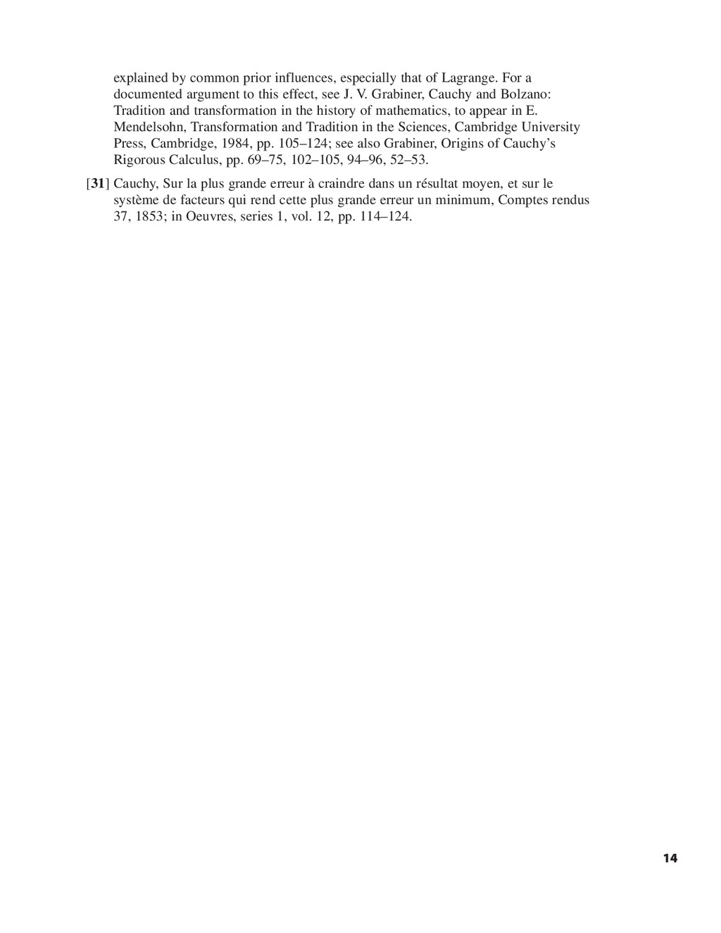
13. [17] Cauchy, op. cit., pp. 378–380. For an English translation of this proof, see Grabiner, Origins, pp. 167–168. For clarity, I have substituted and c, for Cauchy’s and X, in the present version. [18] Lagrange, Equations numériques, sections 2 and 6, in Oeuvres, vol. 8; also in Lagrange, Leçons élémentaires sur les mathématiques données à l’école normale en 1795, Séances des Ecoles Normales, Paris, 1794–1795; in Oeuvres, vol. 7, pp. 181–288; this method is on pp. 260–261. [19] I. Grattan-Guinness, Development of the Foundations of Mathematical Analysis from Euler to Riemann, M. I. T. Press, Cambridge and London, 1970, p. 123, puts it well: “Uniform convergence was tucked away in the word “always,’’ with no reference to the variable at all.’’ [20] Lagrange, Leçons sur le calcul des fonctions, Oeuvres 10, p. 87; compare Lagrange, Théorie des fonctions analytiques, Oeuvres 9, p. 77. I have substituted h for the i Lagrange used for the increment. [21] Lagrange, Théorie des fonctions analytiques, Oeuvres 9, p. 29. Compare Leçons sur le calcul des fonctions, Oeuvres 10, p. 101. For Euler, see his Institutiones calculi differentialis, St. Petersburg, 1755; in Opera, series 1, vol. 10, section 122. [22] Grabiner, Origins of Cauchy’s Rigorous Calculus, chapter 5; also J. V. Grabiner, The origins of Cauchy’s theory of the derivative, Hist. Math., 5, 1978, pp. 379–409. [23] The notation is modernized. For Euler, see Institutiones calculi integralis, St. Petersburg, 1768–1770, 3 vols; in Opera, series 1, vol. 11, p. 184. Eighteenth- century summations approximating integrals are treated in A. P. Iushkevich, O vozniknoveniya poiyatiya ob opredelennom integrale Koshi, Trudy Instituta Istorii Estestvoznaniya, Akademia Nauk SSSR, vol. 1, 1947, pp. 373–411. [24] S. D. Poisson, Suite du mémoire sur les intégrales définies, Journ. de l’Ecole polytechnique, Cah. 18, 11, 1820, pp. 295–341, 319–323. I have substituted h, w for Poisson’s k, and have used for his [25] Poisson, op. cit., pp. 329–330. [26] Cauchy, Cours d’analyse, Introduction, Oeuvres, Series 2, vol. 3, p. iii. [27] Cauchy, Cours d’analyse, Note VIII, Oeuvres, series 2, vol. 3, pp. 456–457. [28] Cauchy, Calcul infinitésimal, Oeuvres, series 2, vol. 4, 122–25; in Grabiner, Origins of Cauchy’s Rigorous Calculus, pp. 171–175 in English translation. [29] Cauchy, op. cit., pp. 151–152. [30] B. Bolzano, Rein analytischer Beweis des Lehrsatzes dass zwischen je zwey Werthen, die ein entgegengesetztes Resultat gewaehren, wenigstens eine reele Wurzel der Gleichung liege, Prague, 1817. English version, S. B. Russ, A translation of Bolzano’s paper on the intermediate value theorem, Hist. Math., 7, 1980, pp. 156–185. The contention by Grattan-Guinness, Foundations, p. 54, that Cauchy took his program of rigorizing analysis, definition of continuity, Cauchy criterion, and proof of the intermediate-value theorem, from Bolzano’s paper without acknowledgement is not, in my opinion, valid; the similarities are better R0 . R1 ␣, XЈЈ, . . . XЈ, x2 , . . . x1 , x0 , c2 , . . . c1 , b2 , . . . b1 , b, 13
14. explained by common prior influences, especially that of Lagrange. For a documented argument to this effect, see J. V. Grabiner, Cauchy and Bolzano: Tradition and transformation in the history of mathematics, to appear in E. Mendelsohn, Transformation and Tradition in the Sciences, Cambridge University Press, Cambridge, 1984, pp. 105–124; see also Grabiner, Origins of Cauchy’s Rigorous Calculus, pp. 69–75, 102–105, 94–96, 52–53. [31] Cauchy, Sur la plus grande erreur à craindre dans un résultat moyen, et sur le système de facteurs qui rend cette plus grande erreur un minimum, Comptes rendus 37, 1853; in Oeuvres, series 1, vol. 12, pp. 114–124. 14