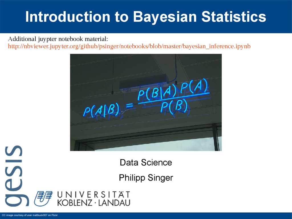
courtesy of user mattbuck007 on Flickr Additional juypter notebook material: http://nbviewer.jupyter.org/github/psinger/notebooks/blob/master/bayesian_inference.ipynb
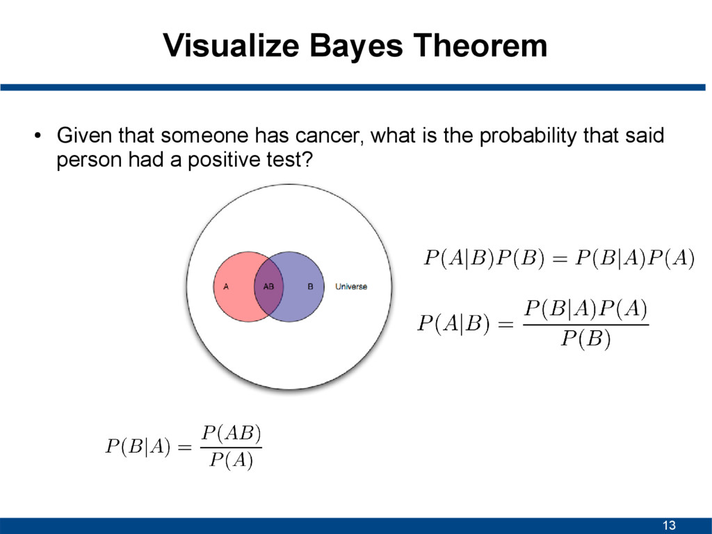
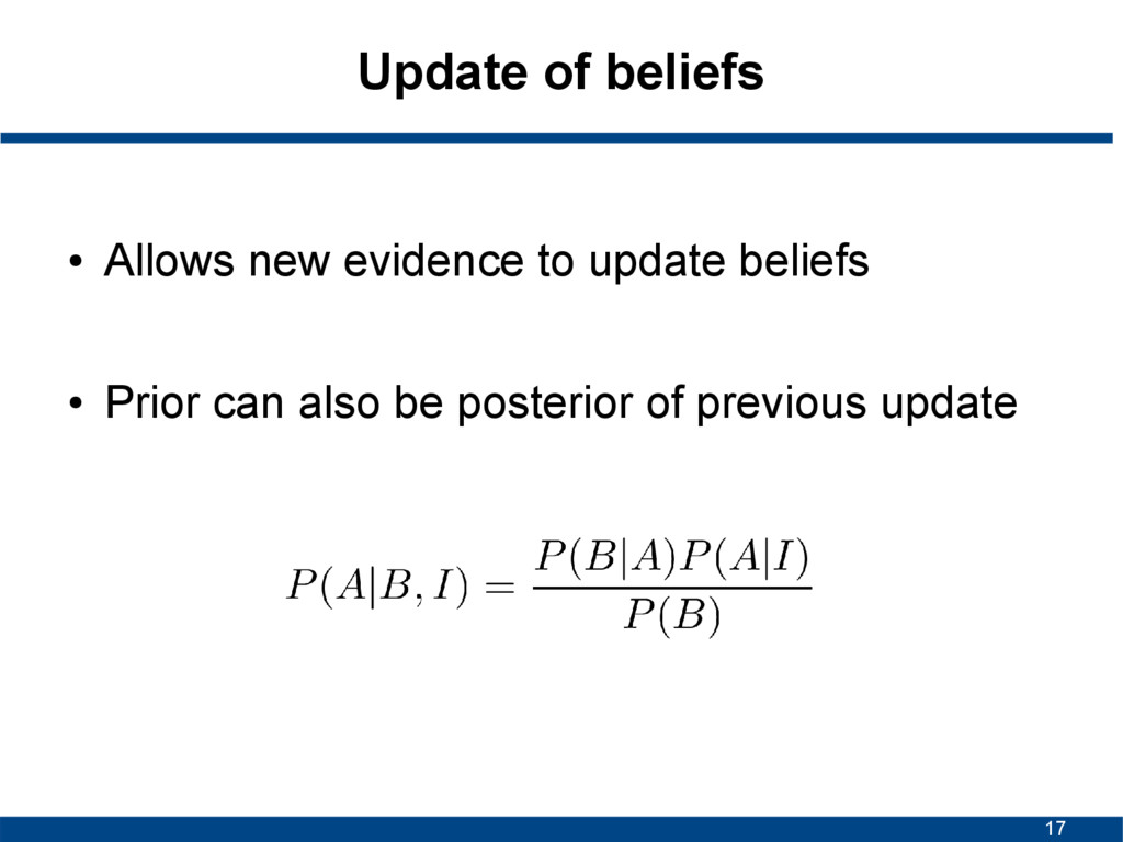
A given B is true • P(B|A) is conditional probability of observing B given A is true • P(A) and P(B) are probabilities of A and B without conditioning on each other
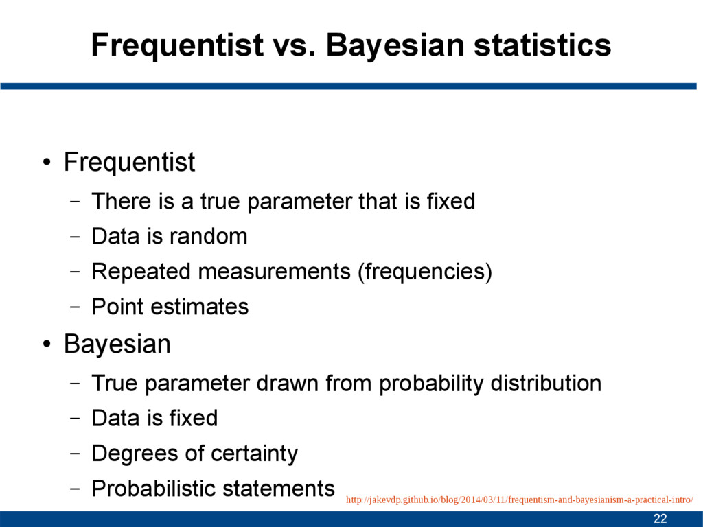
a true parameter that is fixed – Data is random – Repeated measurements (frequencies) – Point estimates • Bayesian – True parameter drawn from probability distribution – Data is fixed – Degrees of certainty – Probabilistic statements http://jakevdp.github.io/blog/2014/03/11/frequentism-and-bayesianism-a-practical-intro/
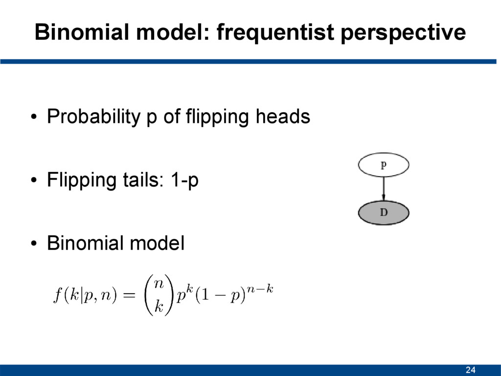
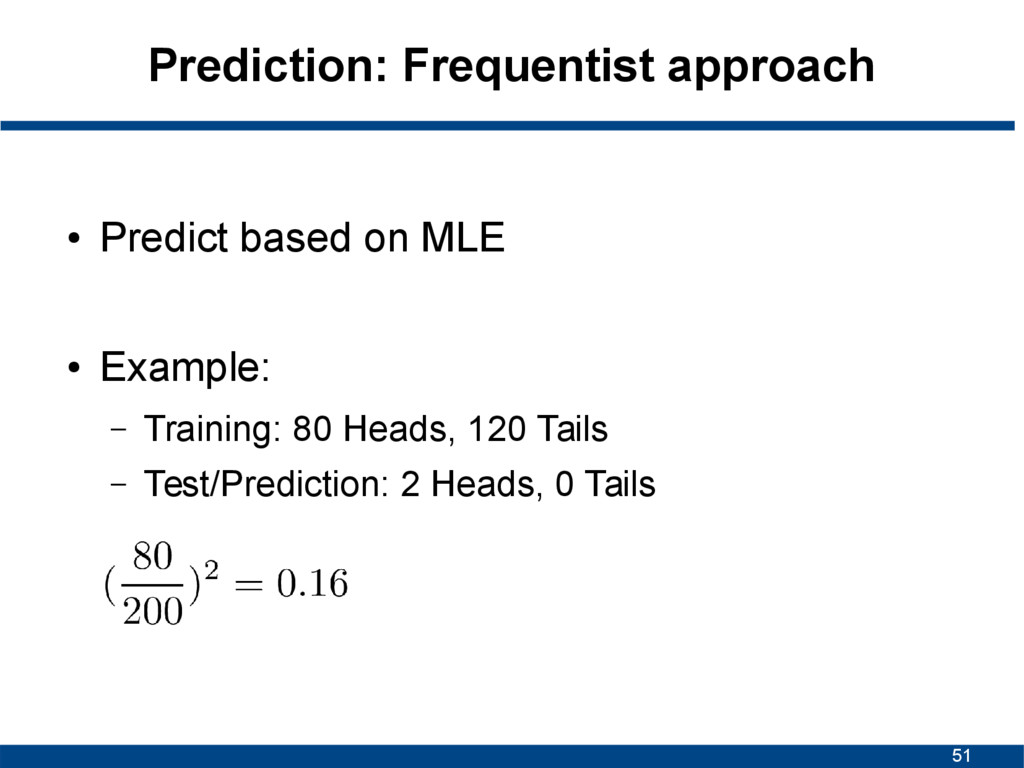
is random • Find estimate for parameter (point estimate) • Maximum likelihood estimation (MLE) – Estimate parameter by maximizing likelihood – Covered in previous lectures
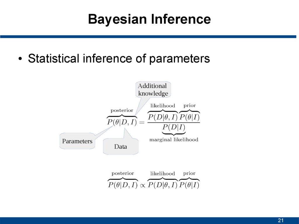
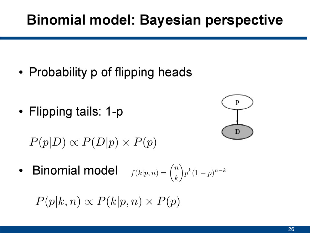
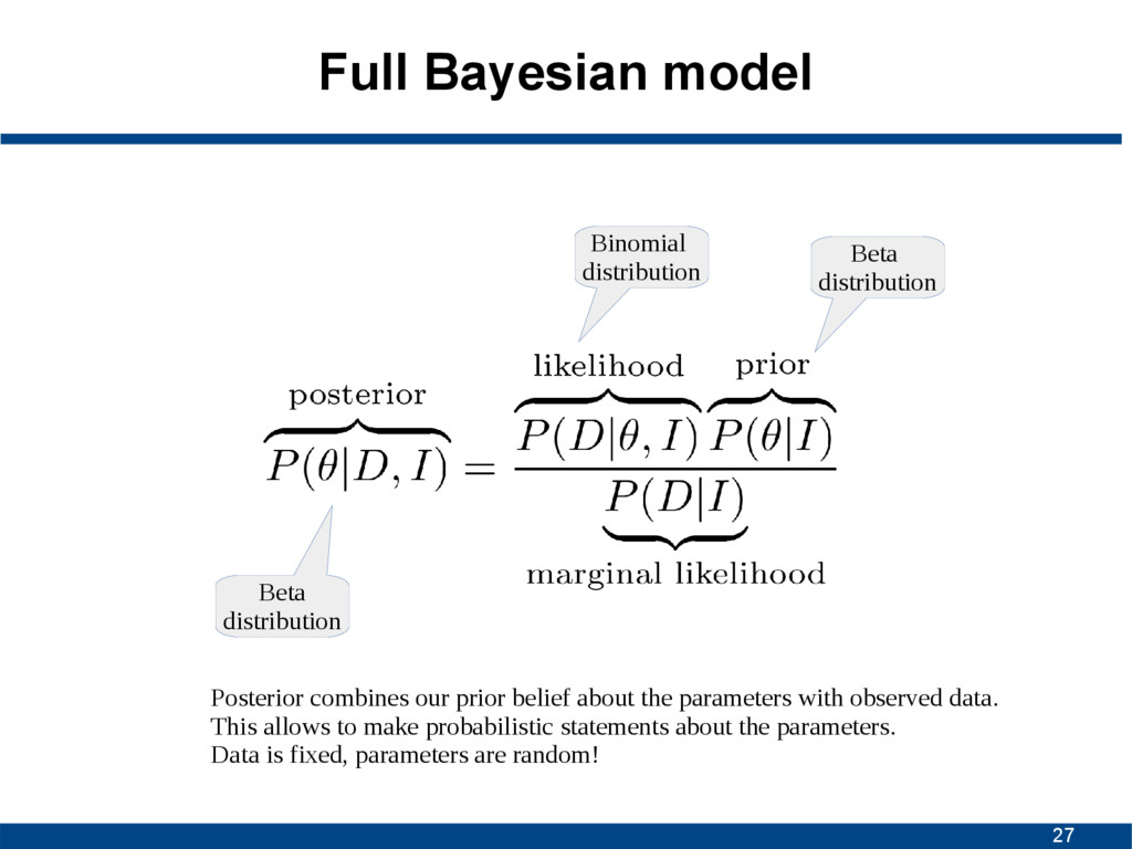
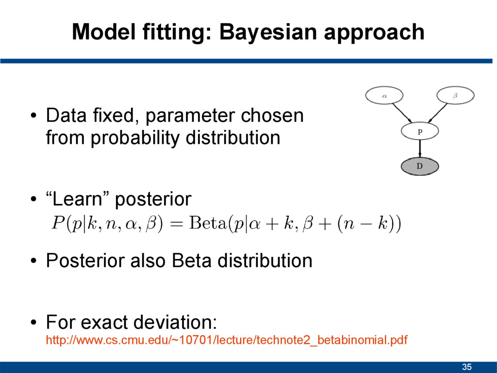
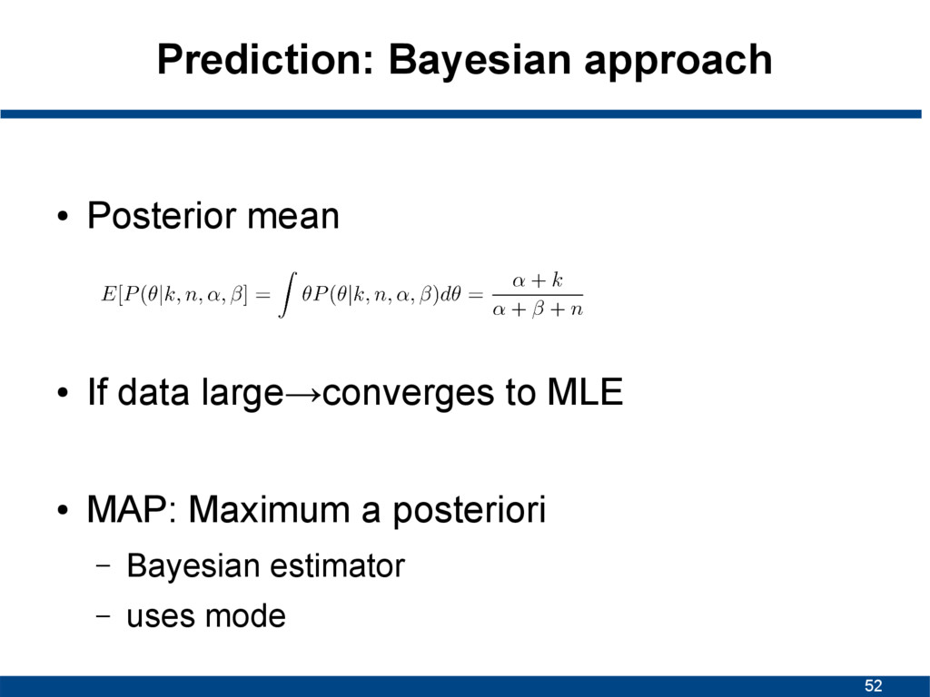
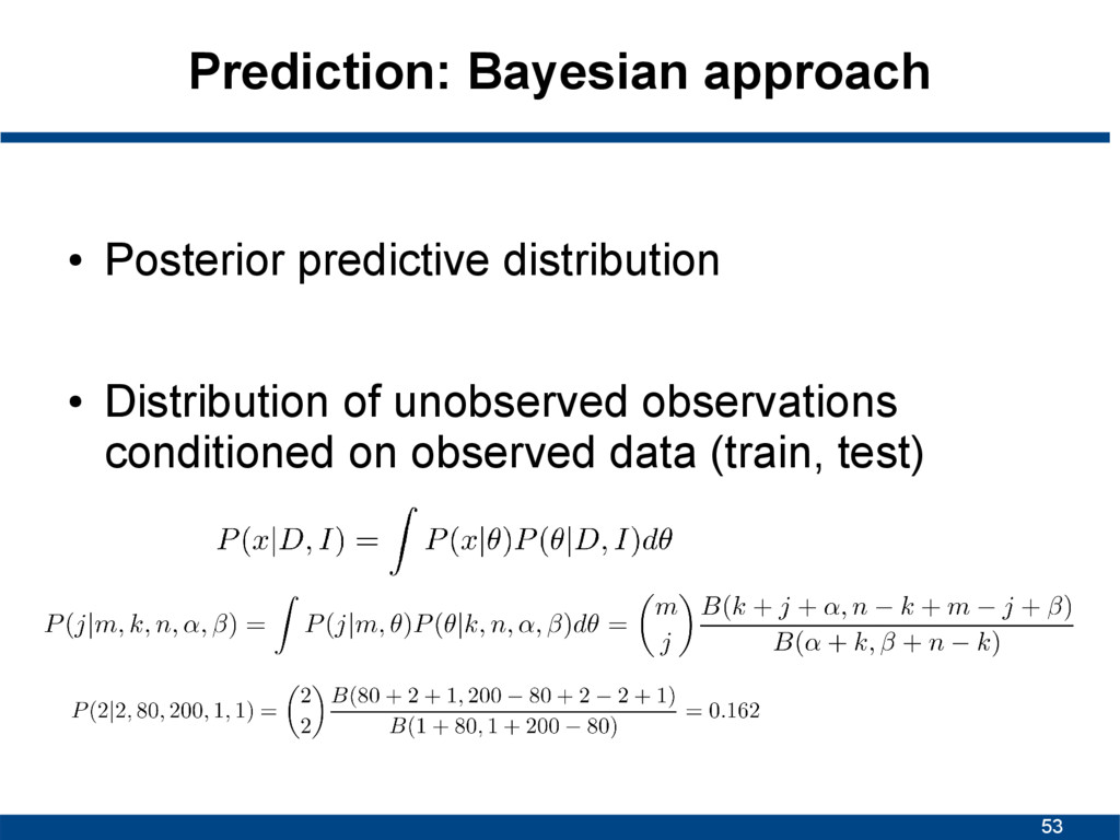
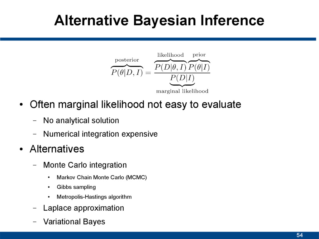
Posterior combines our prior belief about the parameters with observed data. This allows to make probabilistic statements about the parameters. Data is fixed, parameters are random!
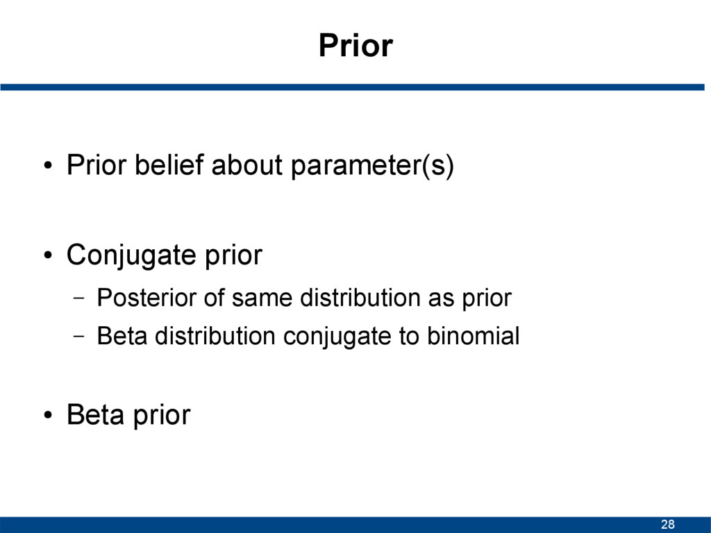
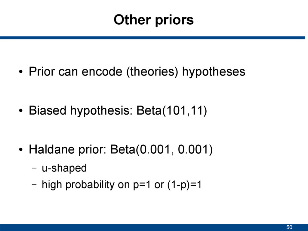
from probability distribution • “Learn” posterior • Posterior also Beta distribution • For exact deviation: http://www.cs.cmu.edu/~10701/lecture/technote2_betabinomial.pdf
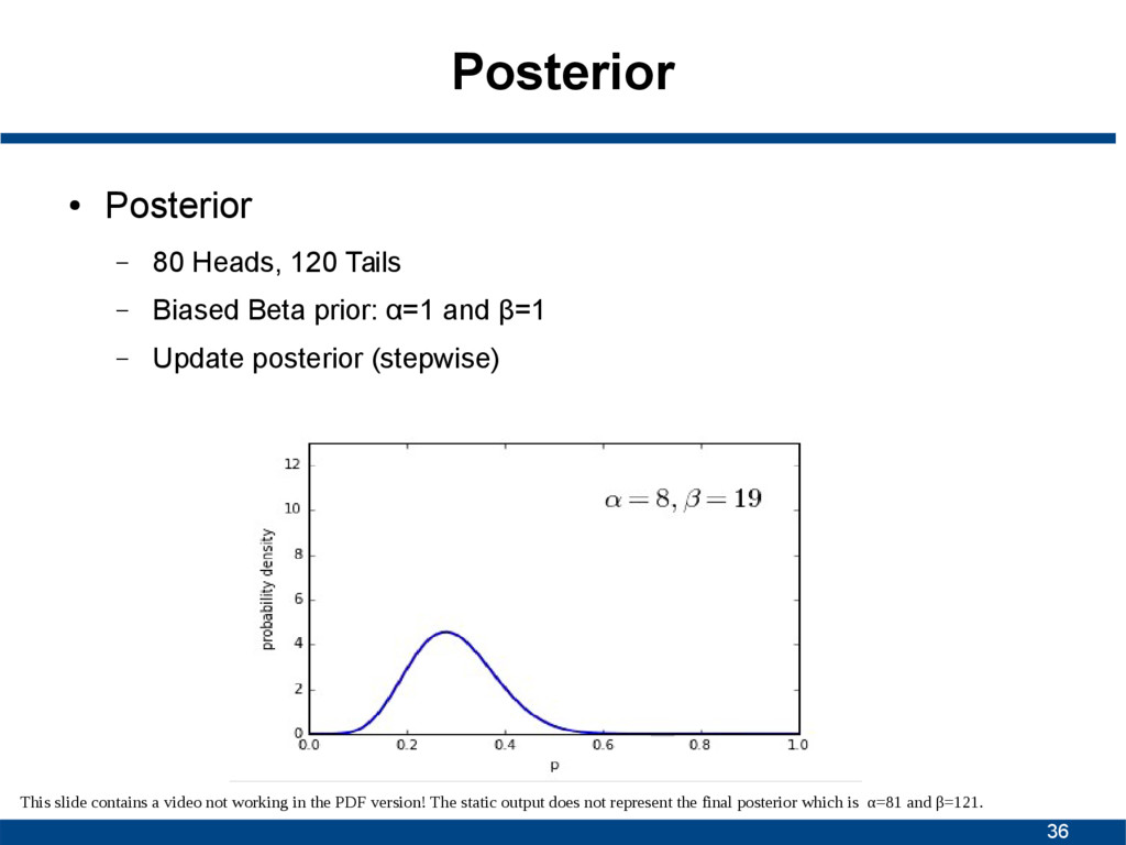
Biased Beta prior: α=1 and β=1 – Update posterior (stepwise) This slide contains a video not working in the PDF version! The static output does not represent the final posterior which is α=81 and β=121.
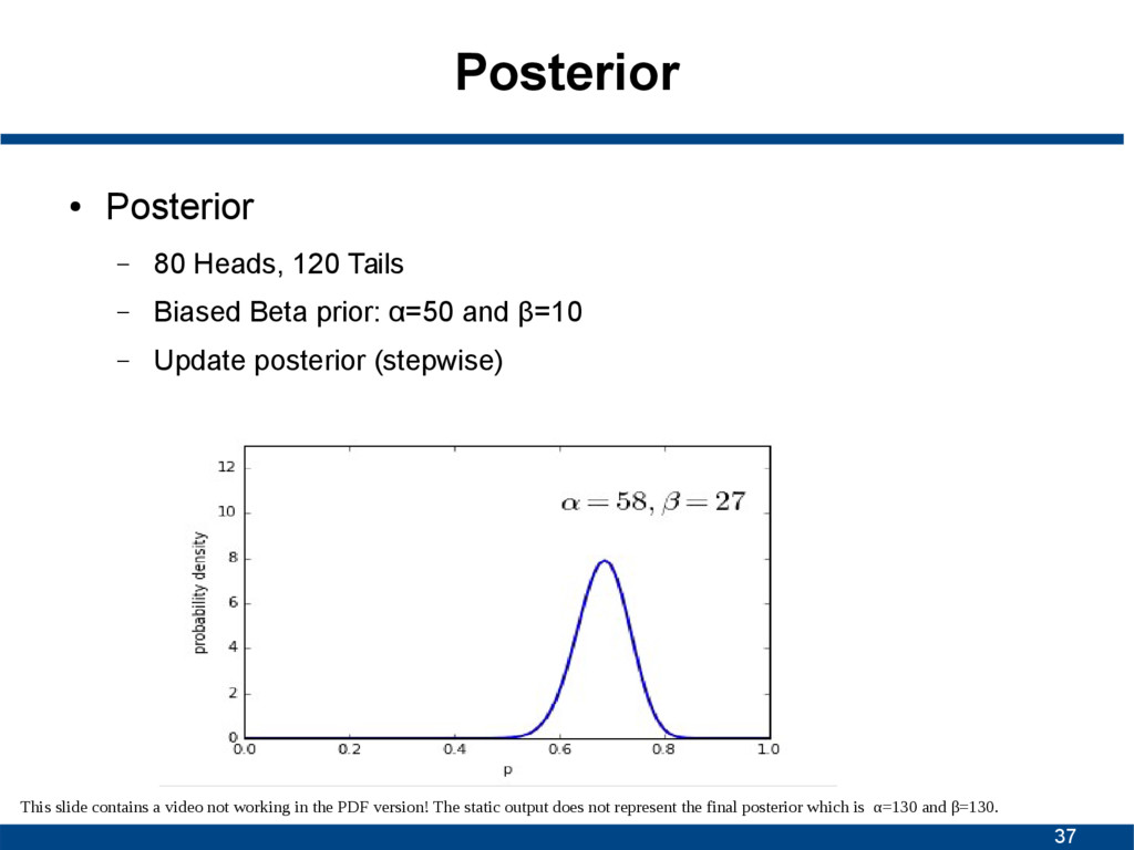
Biased Beta prior: α=50 and β=10 – Update posterior (stepwise) This slide contains a video not working in the PDF version! The static output does not represent the final posterior which is α=130 and β=130.
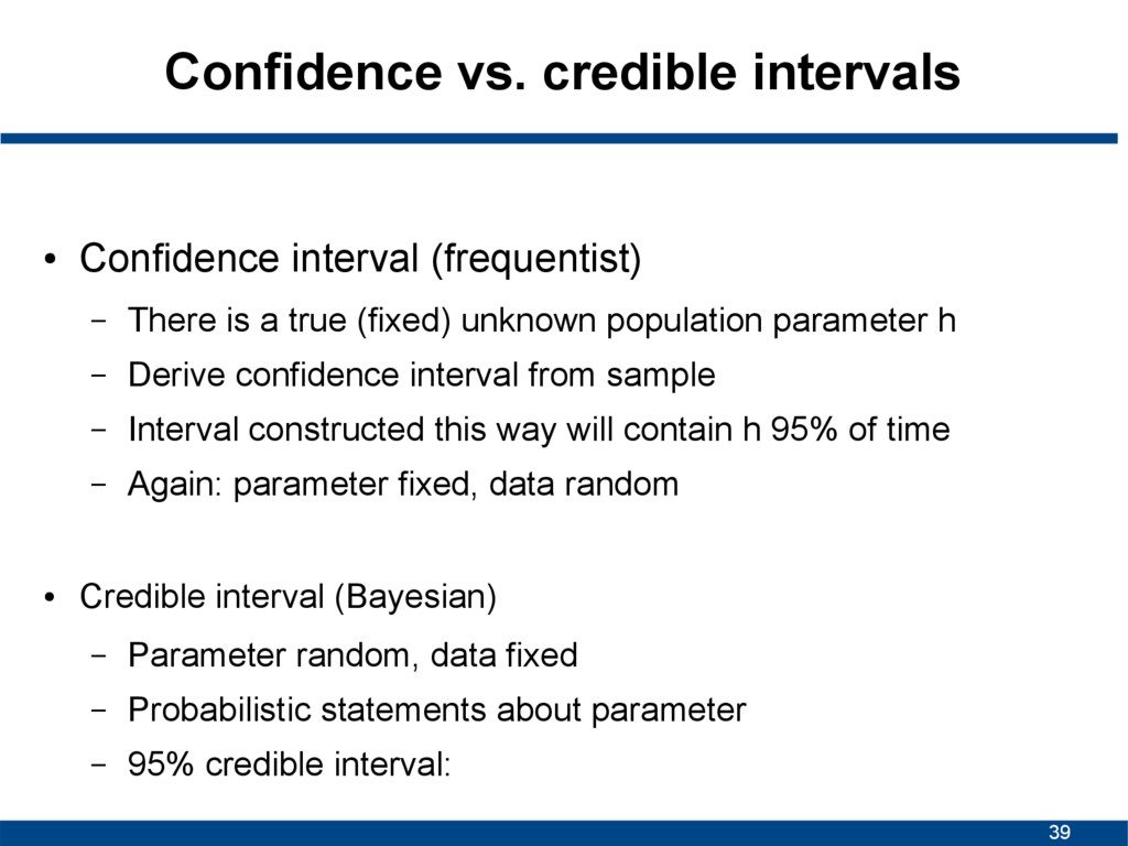
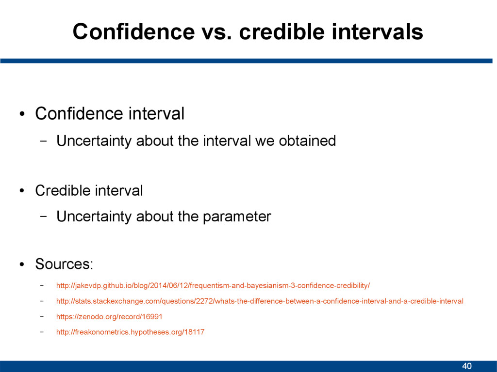
There is a true (fixed) unknown population parameter h – Derive confidence interval from sample – Interval constructed this way will contain h 95% of time – Again: parameter fixed, data random • Credible interval (Bayesian) – Parameter random, data fixed – Probabilistic statements about parameter – 95% credible interval:
about the interval we obtained • Credible interval – Uncertainty about the parameter • Sources: – http://jakevdp.github.io/blog/2014/06/12/frequentism-and-bayesianism-3-confidence-credibility/ – http://stats.stackexchange.com/questions/2272/whats-the-difference-between-a-confidence-interval-and-a-credible-interval – https://zenodo.org/record/16991 – http://freakonometrics.hypotheses.org/18117
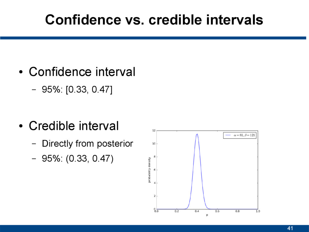
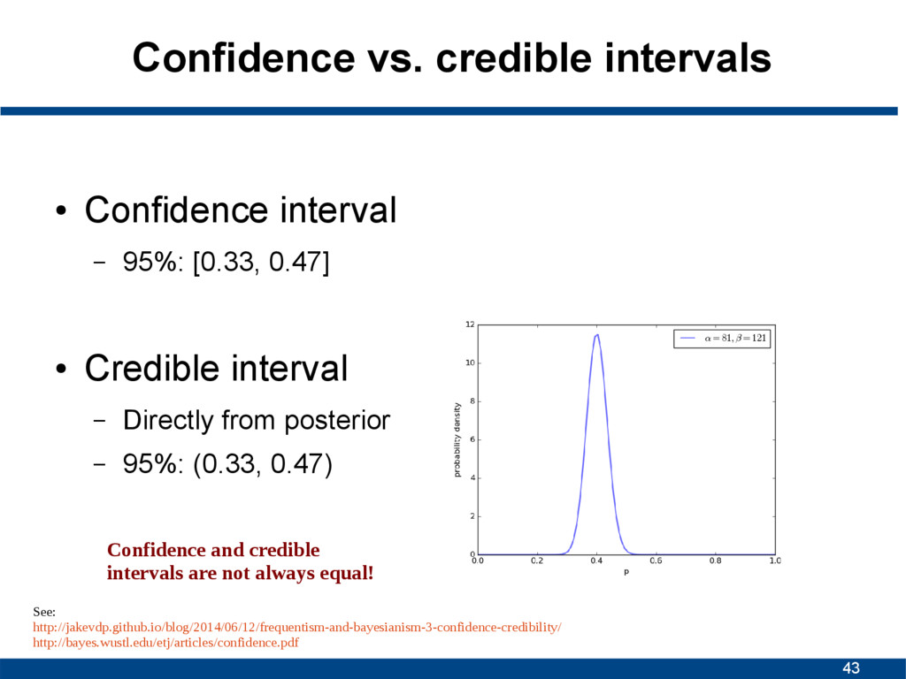
[0.33, 0.47] • Credible interval – Directly from posterior – 95%: (0.33, 0.47) Given observed data, there is a 95% probability that the true value of p falls within credible interval There is a 95% probability that when I create confidence intervals of this sort, the CI will include the population parameter p.
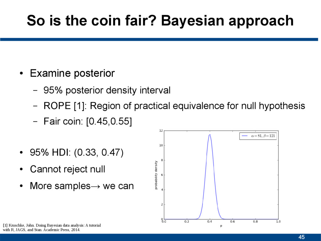
posterior – 95% posterior density interval – ROPE [1]: Region of practical equivalence for null hypothesis – Fair coin: [0.45,0.55] • 95% HDI: (0.33, 0.47) • Cannot reject null • More samples→ we can [1] Kruschke, John. Doing Bayesian data analysis: A tutorial with R, JAGS, and Stan. Academic Press, 2014.
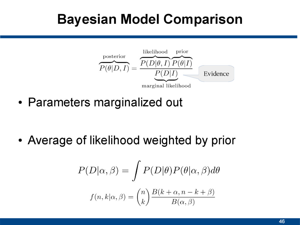
of marginal likelihoods • Interpretation table by Kass & Raftery [1] • >100 → decisive evidence against M2 [1] Kass, Robert E., and Adrian E. Raftery. "Bayes factors." Journal of the american statistical association 90.430 (1995): 773-795.
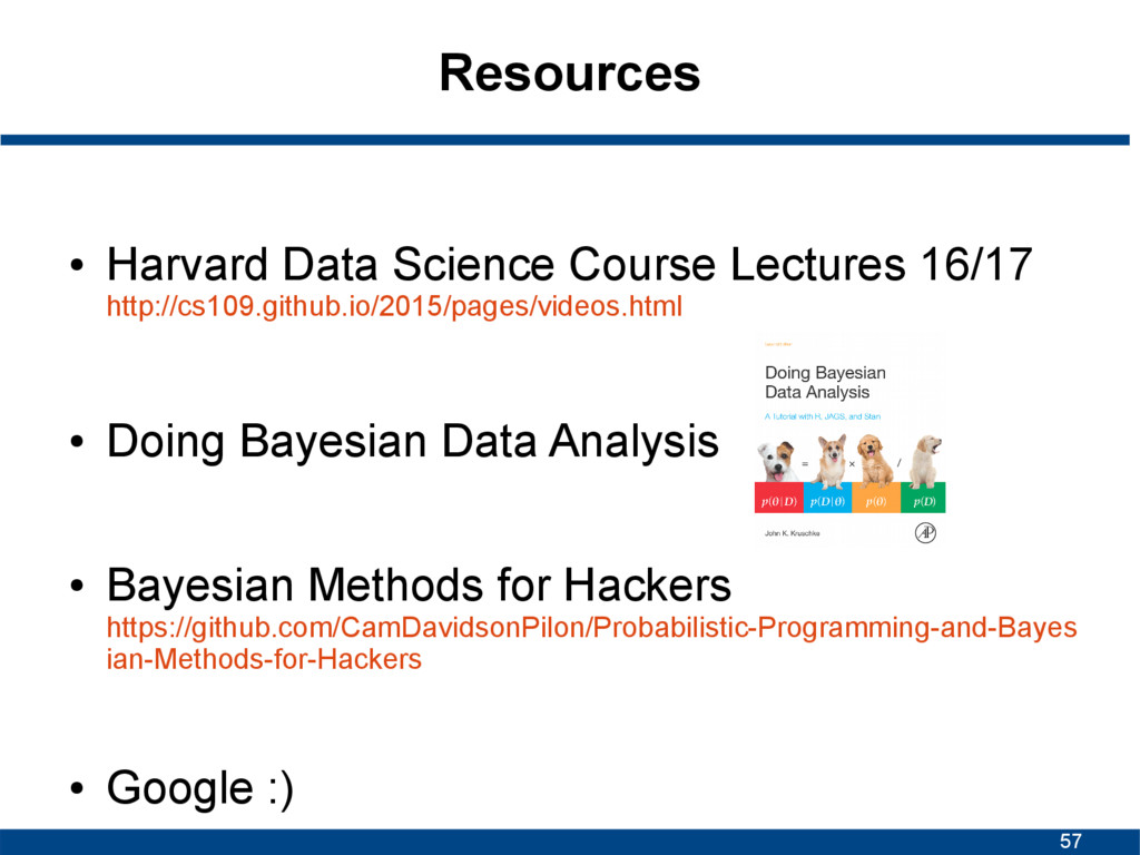
• Doing Bayesian Data Analysis • Bayesian Methods for Hackers https://github.com/CamDavidsonPilon/Probabilistic-Programming-and-Bayes ian-Methods-for-Hackers • Google :)
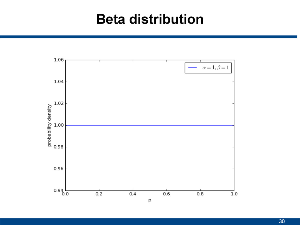
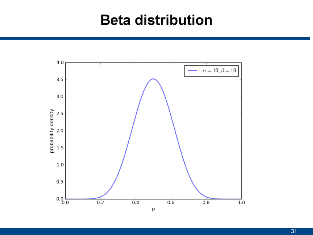
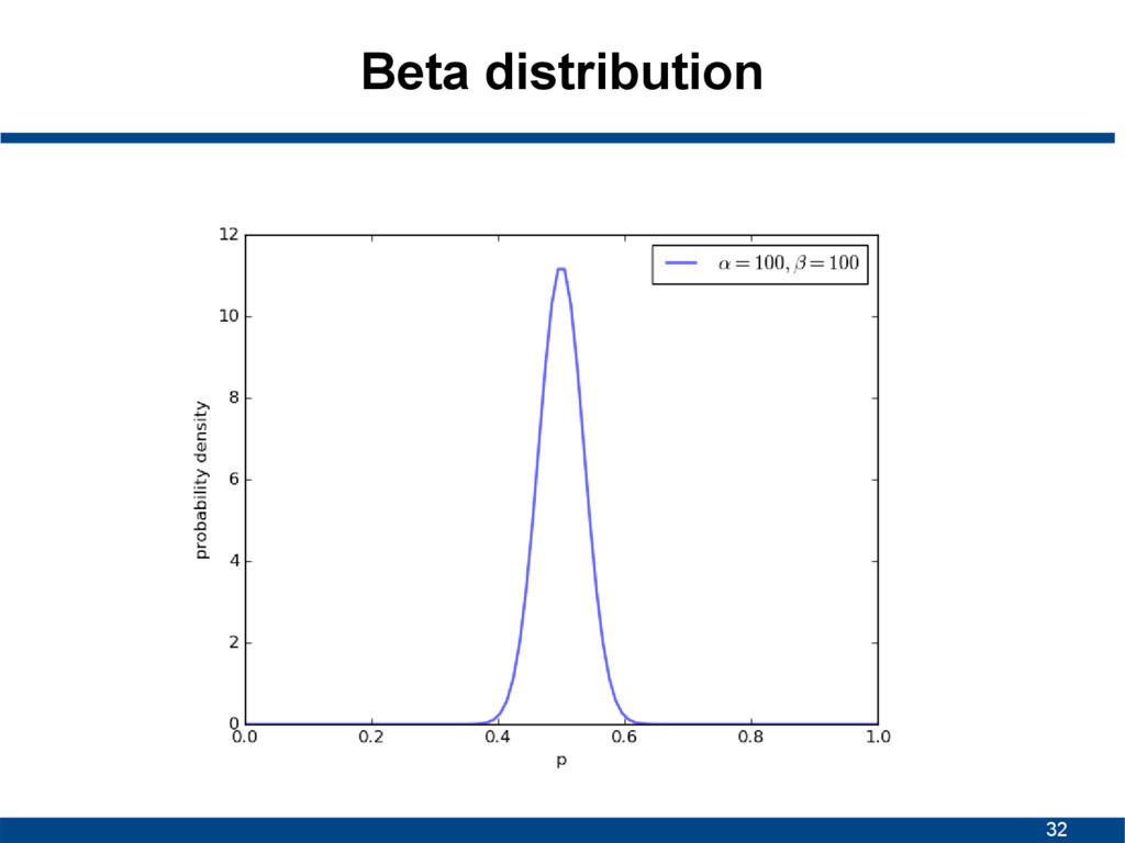
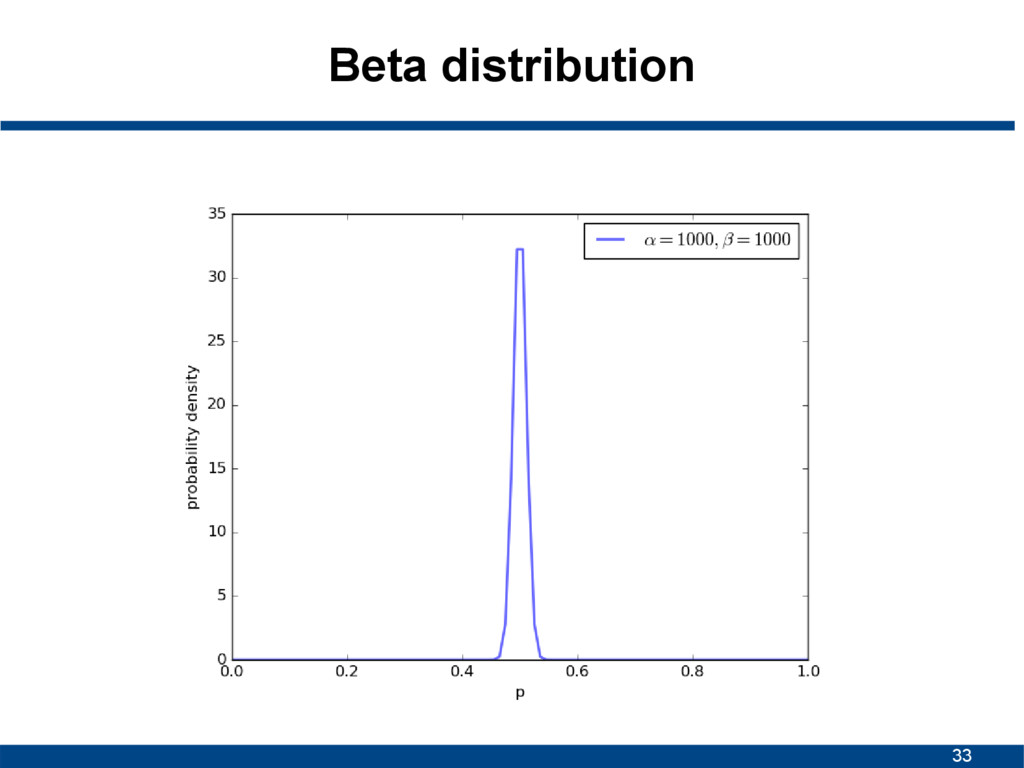
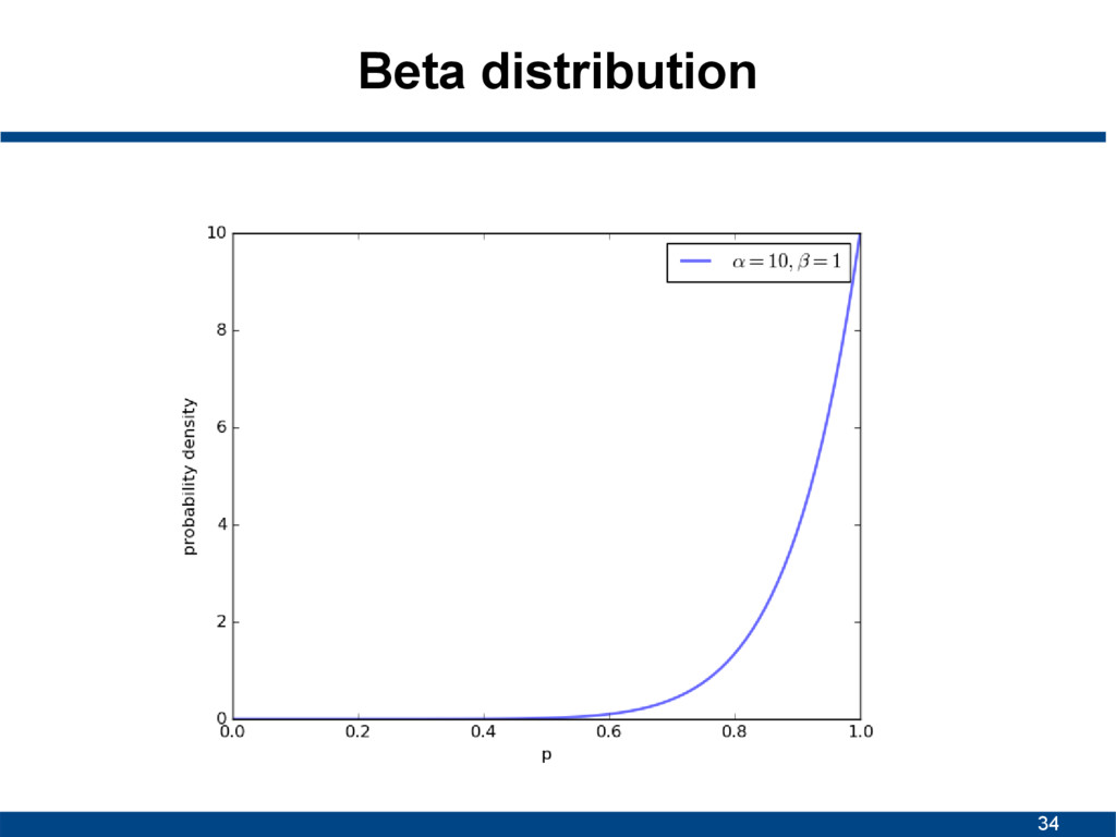
![29 Beta distribution • Continuous probability distribution • Interval [0,1]](https://files.speakerdeck.com/presentations/78528ac31f4c467c866cd1e20ce32750/slide_28.jpg)
![47 Bayesian Model Comparison • Bayes factors [1] • Ratio](https://files.speakerdeck.com/presentations/78528ac31f4c467c866cd1e20ce32750/slide_46.jpg)
![59 Questions? Philipp Singer [email protected] Image credit: talk of Mike](https://files.speakerdeck.com/presentations/78528ac31f4c467c866cd1e20ce32750/slide_58.jpg)