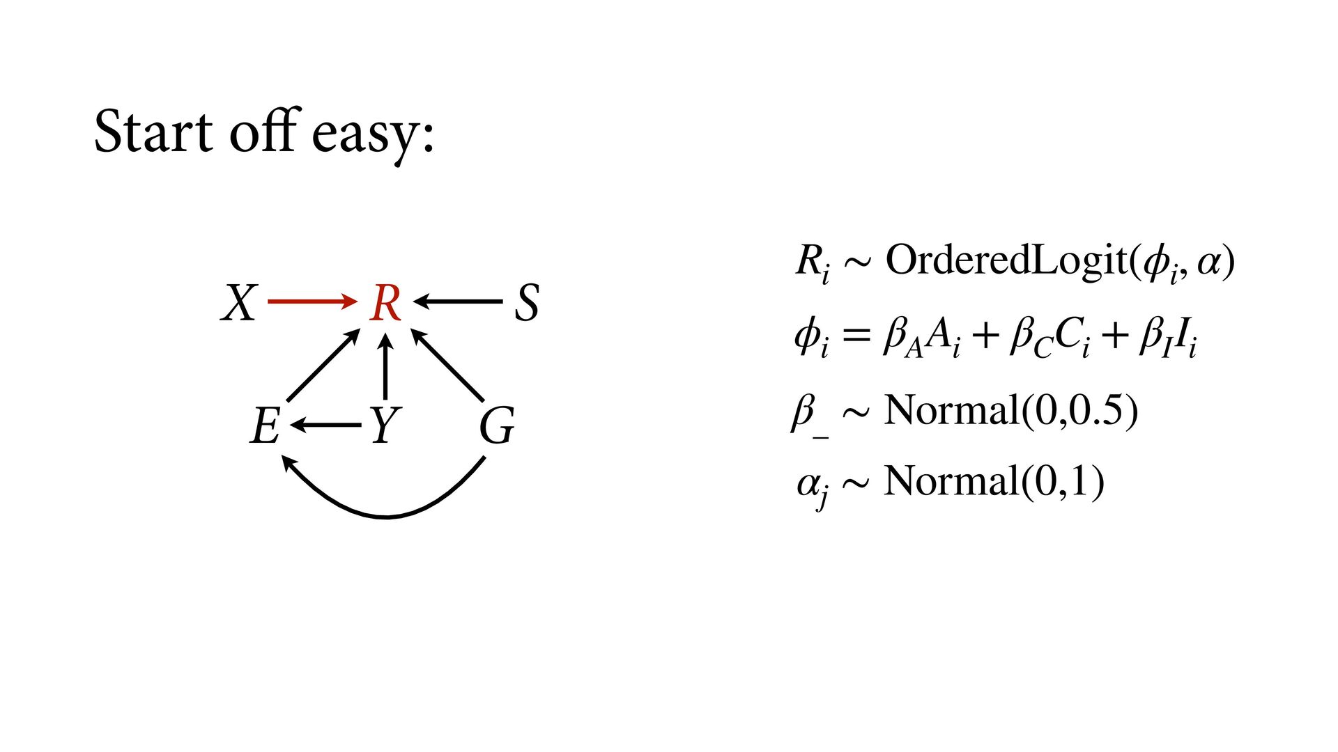
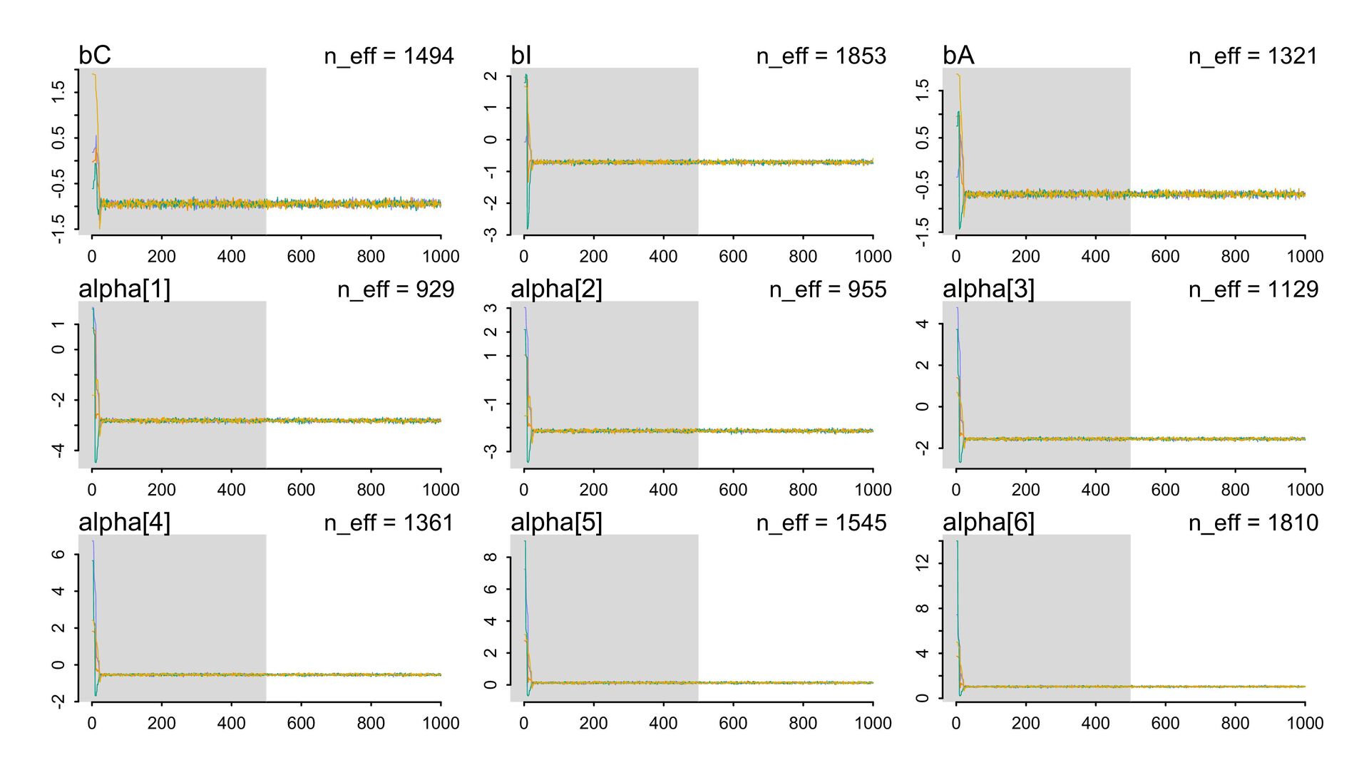
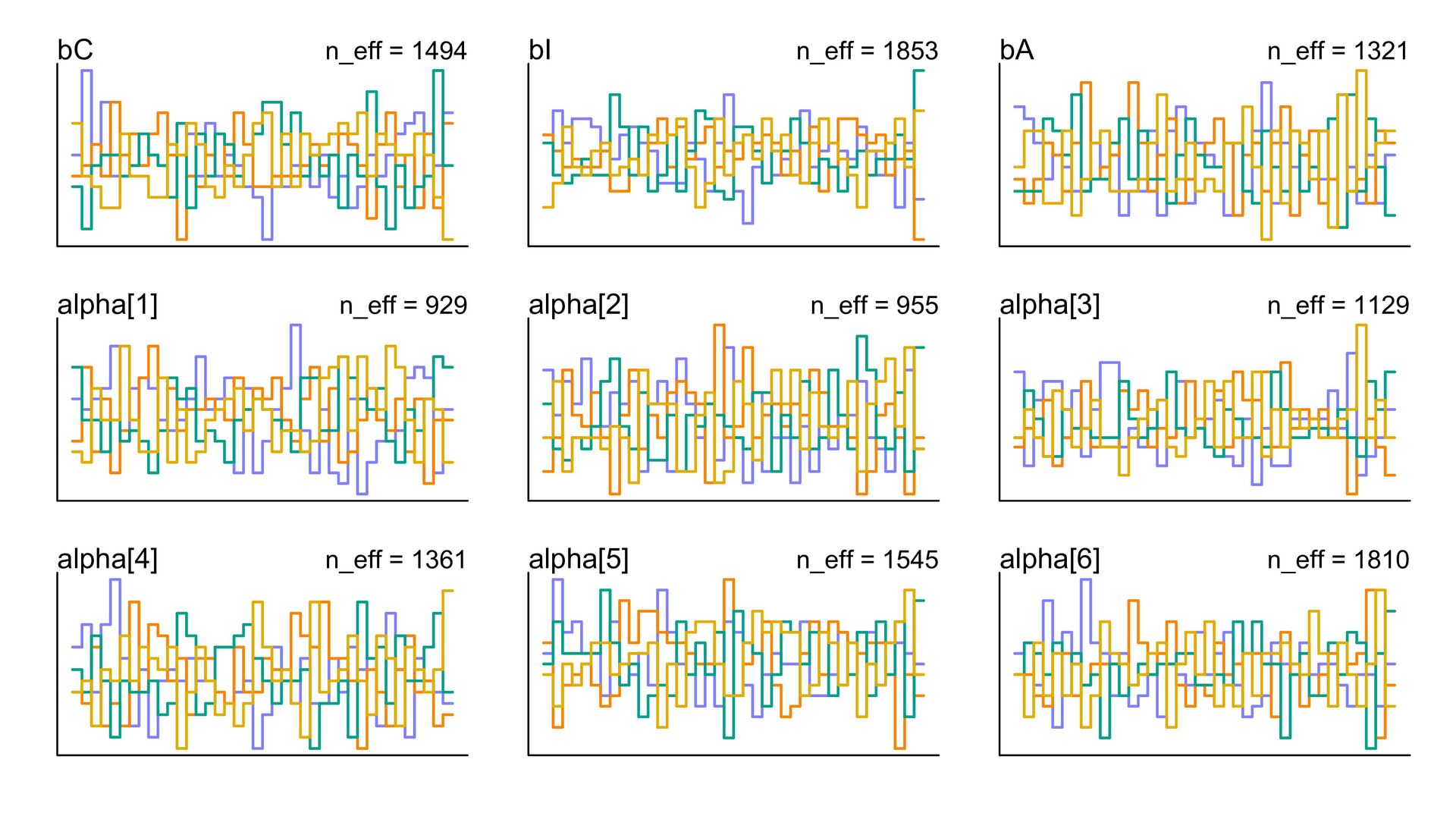
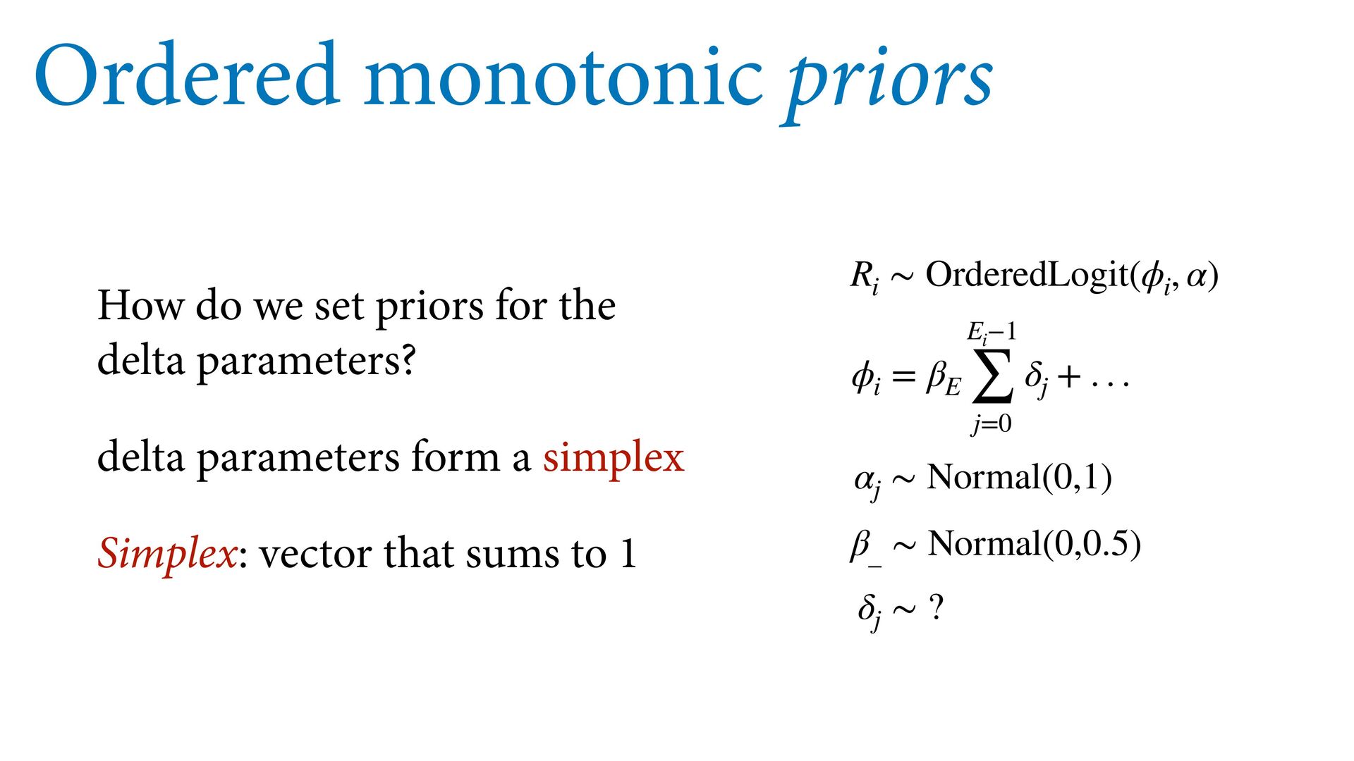
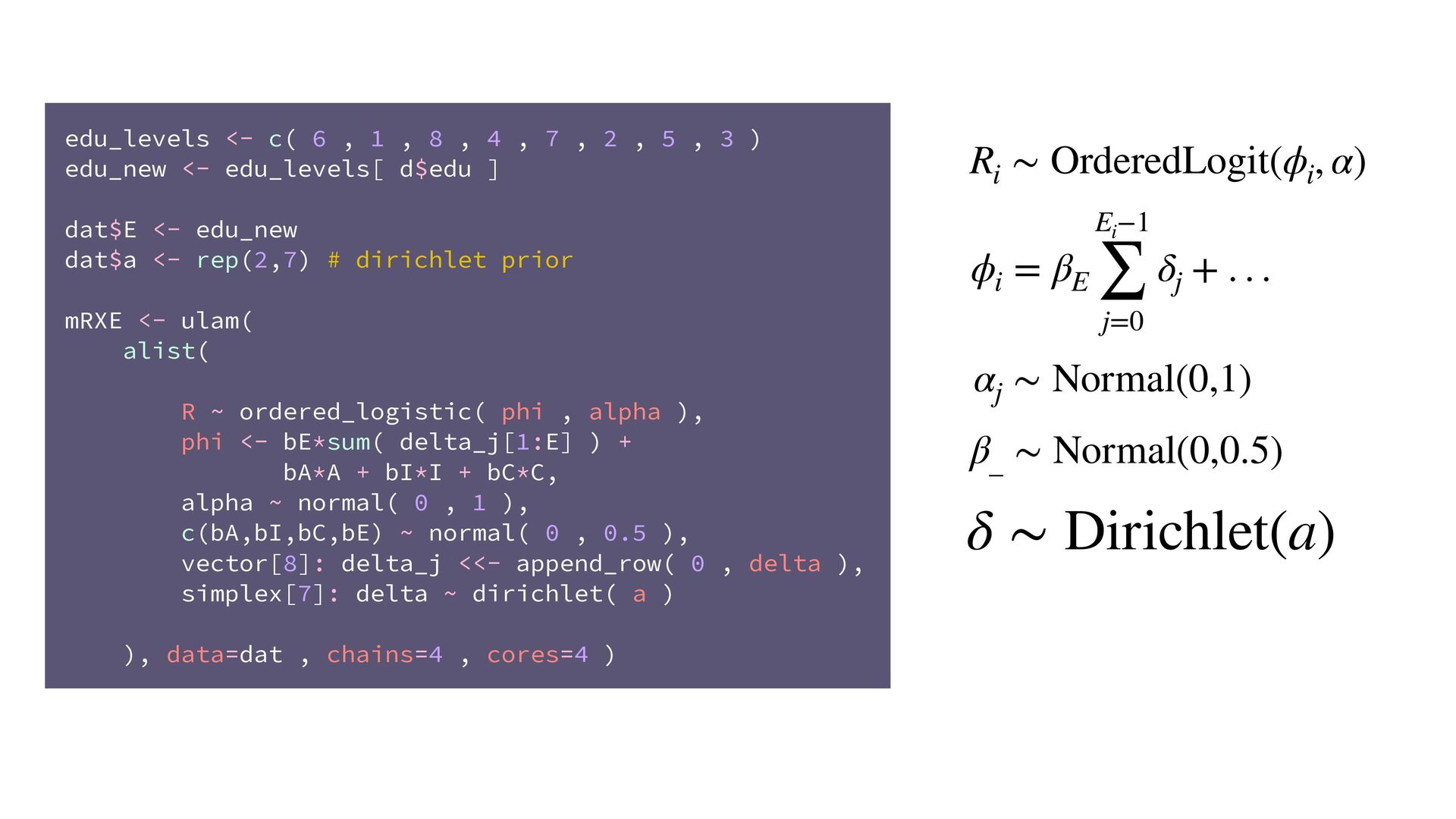
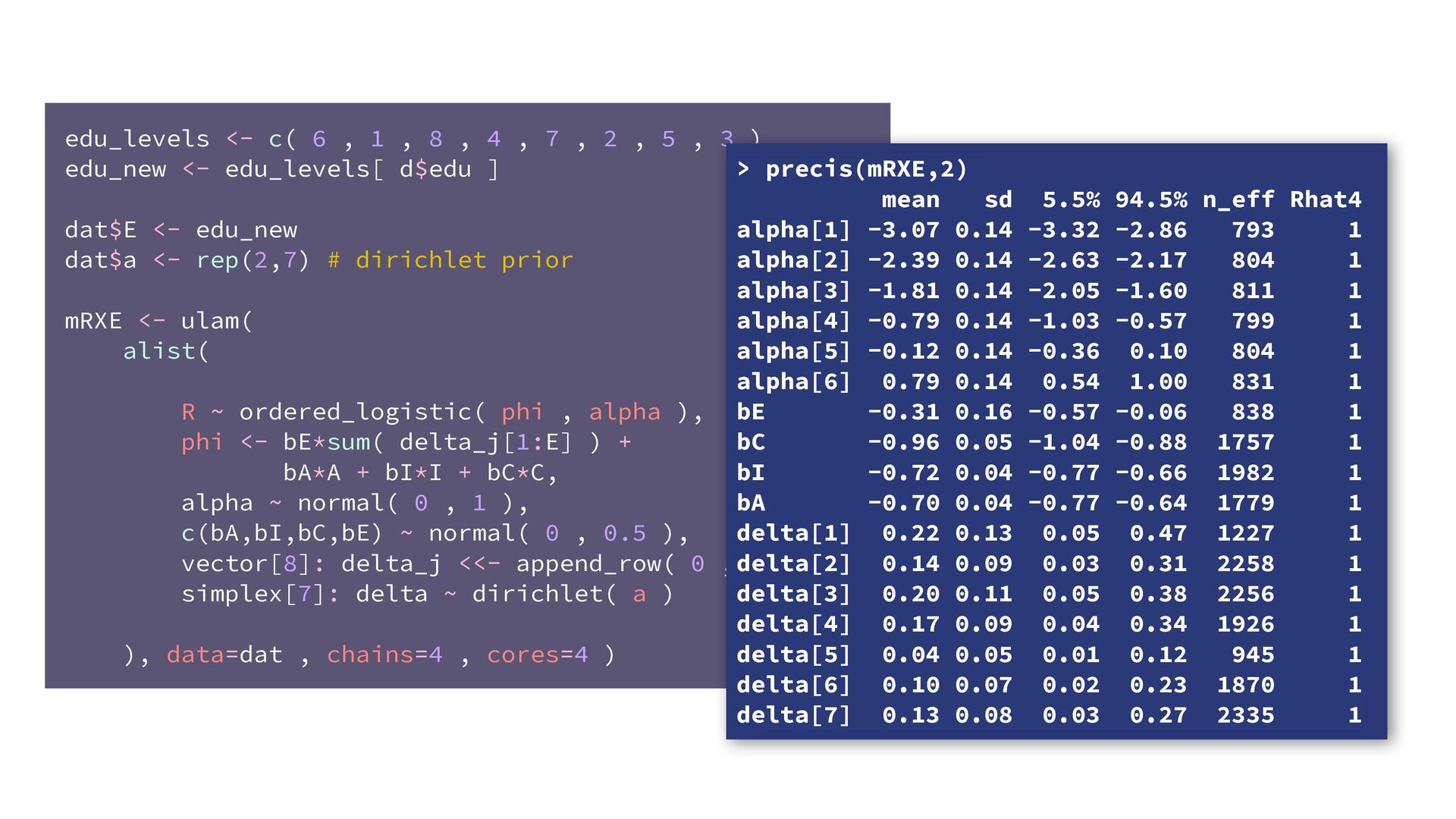
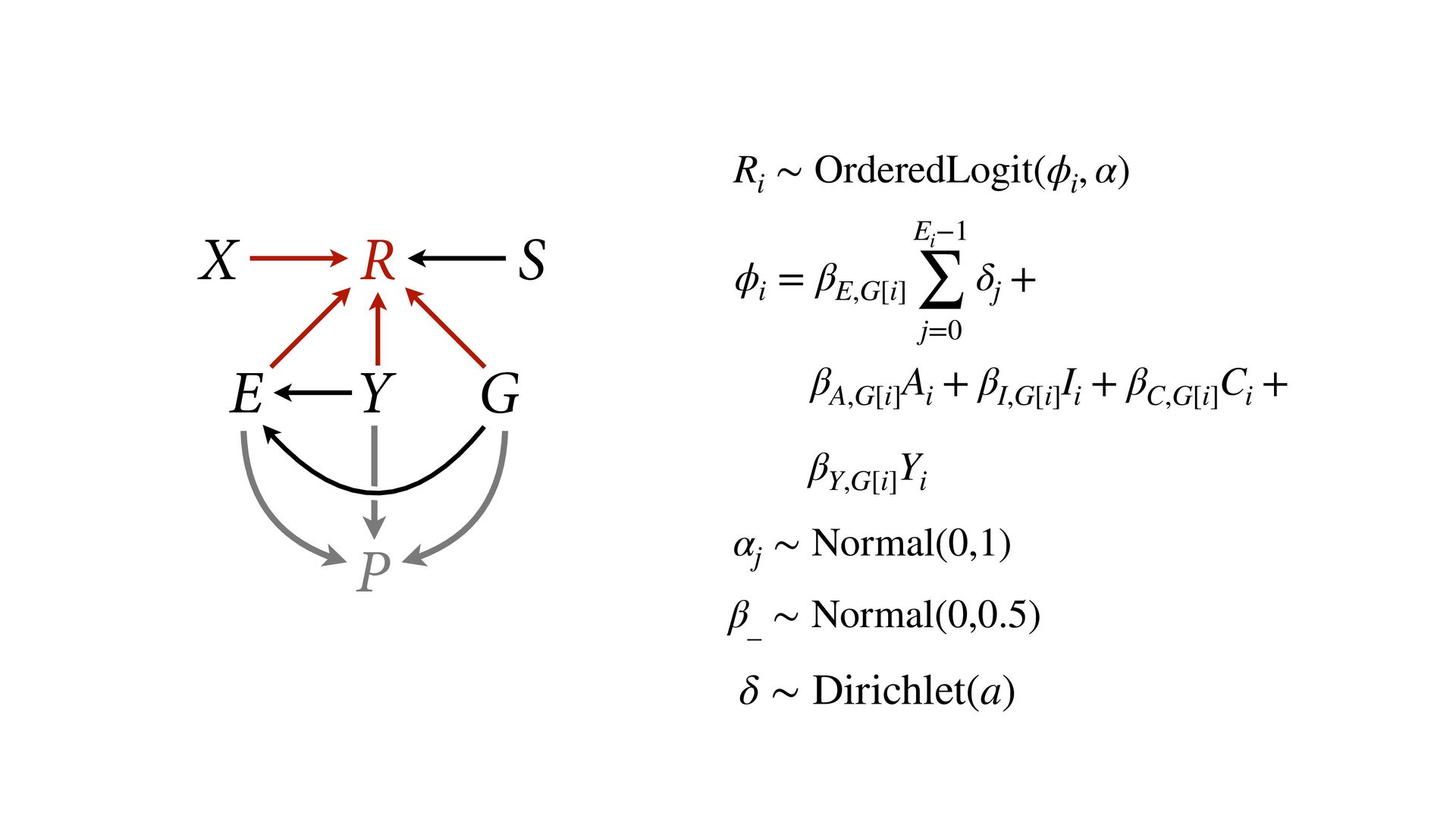
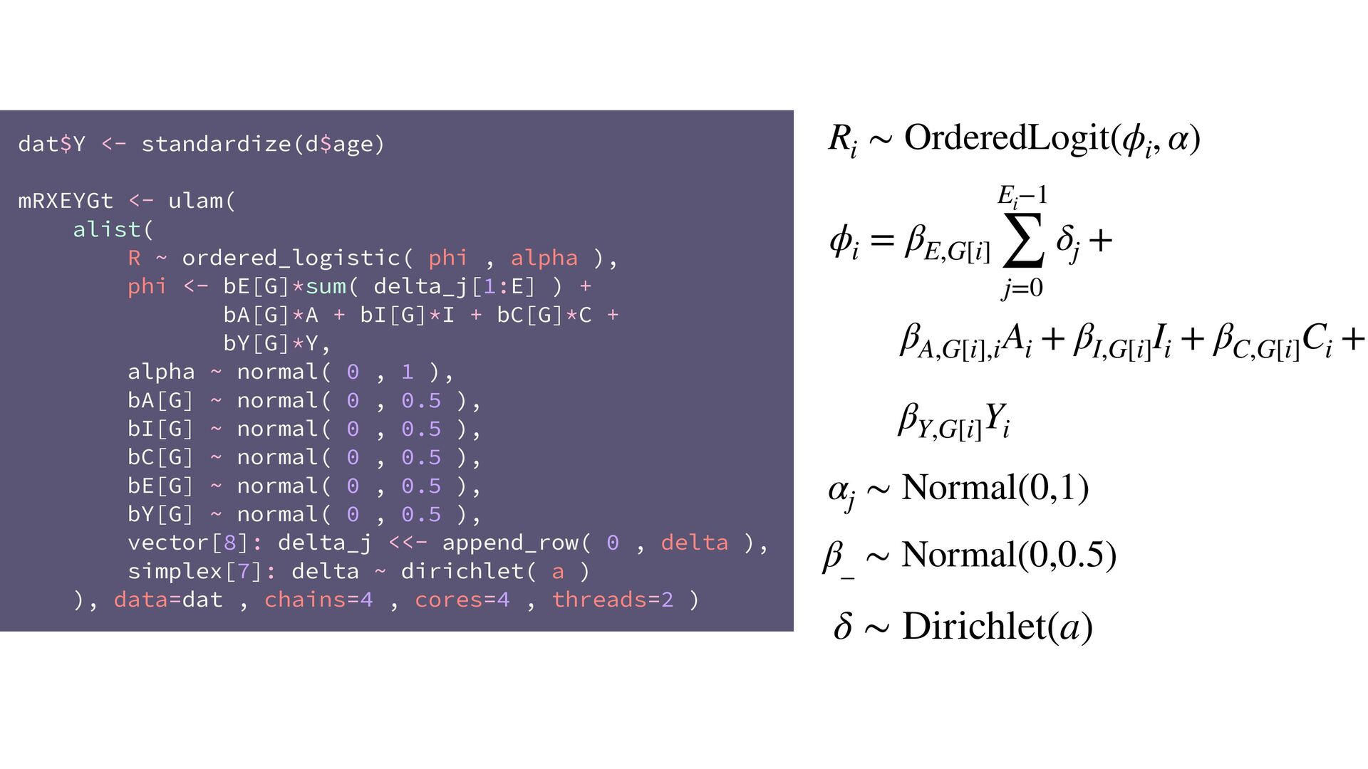
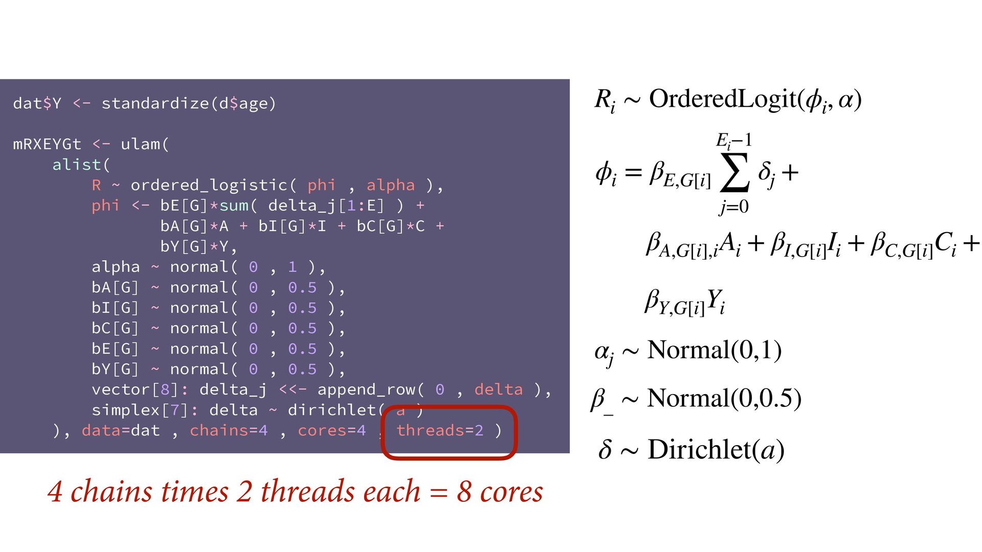
phi , alpha ), phi <- bE[G]*sum( delta_j[1:E] ) + bA[G]*A + bI[G]*I + bC[G]*C + bY[G]*Y, alpha ~ normal( 0 , 1 ), bA[G] ~ normal( 0 , 0.5 ), bI[G] ~ normal( 0 , 0.5 ), bC[G] ~ normal( 0 , 0.5 ), bE[G] ~ normal( 0 , 0.5 ), bY[G] ~ normal( 0 , 0.5 ), vector[8]: delta_j <<- append_row( 0 , delta ), simplex[7]: delta ~ dirichlet( a ) ), data=dat , chains=4 , cores=4 , threads=2 ) δ ∼ Dirichlet(a) ϕ i = β E,G[i] E i −1 ∑ j= 0 δ j + . R i ∼ OrderedLogit(ϕ i , α) α j ∼ Normal(0,1) β _ ∼ Normal(0,0.5) β A,G[i],i A i + β I,G[i] I i + β C,G[i] C i + β Y,G[i] Y i 4 chains times 2 threads each = 8 cores
![δ ∼ Dirichlet(a) a = [2,2,2,2,2,2,2] δ ∼ Dirichlet(a) a](https://files.speakerdeck.com/presentations/96715b386cd147c48bd6db4c93c17fdc/slide_55.jpg)
![δ ∼ Dirichlet(a) a = [2,2,2,2,2,2,2] δ ∼ Dirichlet(a) a](https://files.speakerdeck.com/presentations/96715b386cd147c48bd6db4c93c17fdc/slide_56.jpg)