Python & Machine Learning in Agronomy - Pycon Co 2025 EAFIT

Transcript

1. The Digital Agronomist Juan David Roa Valencia
2. Who am I? • Software Engineer, MSc in CS 󰞐 • Nerd 🧠 🤓 • Vintage cameras lover 📷 🎞 • Nature hiker/lover 🌿 • Open source contributor 🐧 • Rails Girls Cali Co-organizer • Biker 🚲 🏍 • Cat person 🐈
3. Project Members Camilo Estrella Villarreal – Civil Engineer, MSc in Data Analysis Juan Roa – Software Engineer, MSc in Computer Science. Dr. Aicardo Roa-Espinosa – CEO Soilnet LLC Sue Byram – Financial Officer Soilnet LLC Dr. Hien Nguyen – Project Advisor Michelle Pham – MSc in Environmental Science Camilo Perez – PhD in Mechanical Engineering Samuel Roa-Lauby, Lab Manager Soilnet LLC Alexander Seyfarth – Global XRF Technology Manager at SGS Tatiana Quiñonez – Mathematics, MSc in Statistics
5. Plant analysis
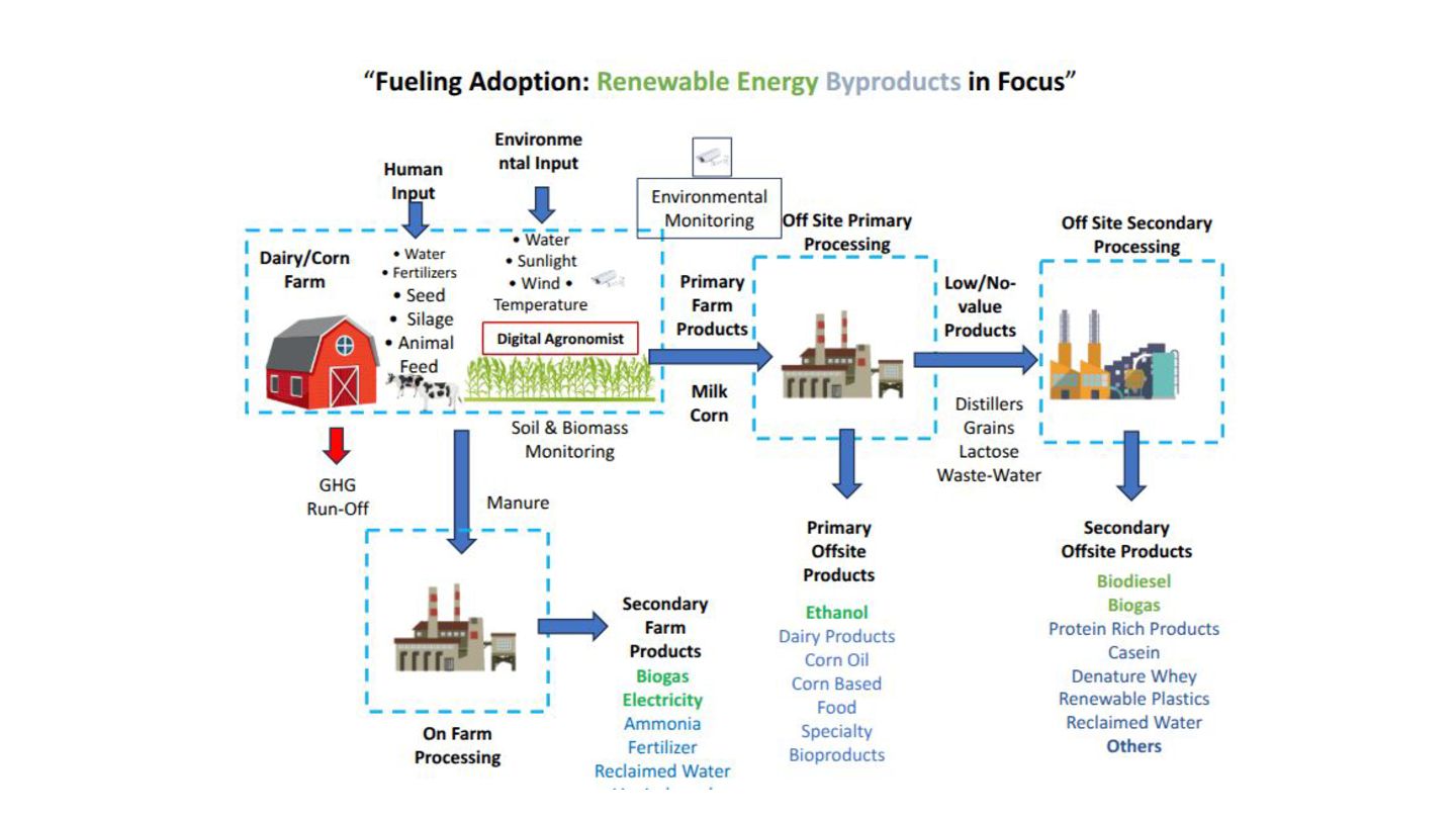
6. Motivation • Agriculture remains a cornerstone of global economies, heavily reliant on continuous technological advancements for sustainability and efficiency. • Challenges: The industry grapples with high costs and complexities in soil nutrient analysis, directly hampers optimal agricultural productivity. • By reducing the costs associated with nutrient analysis and improving data accuracy, this initiative aims to enhance crop yield predictions and soil management—paving the way for more innovative, economical agricultural practices.
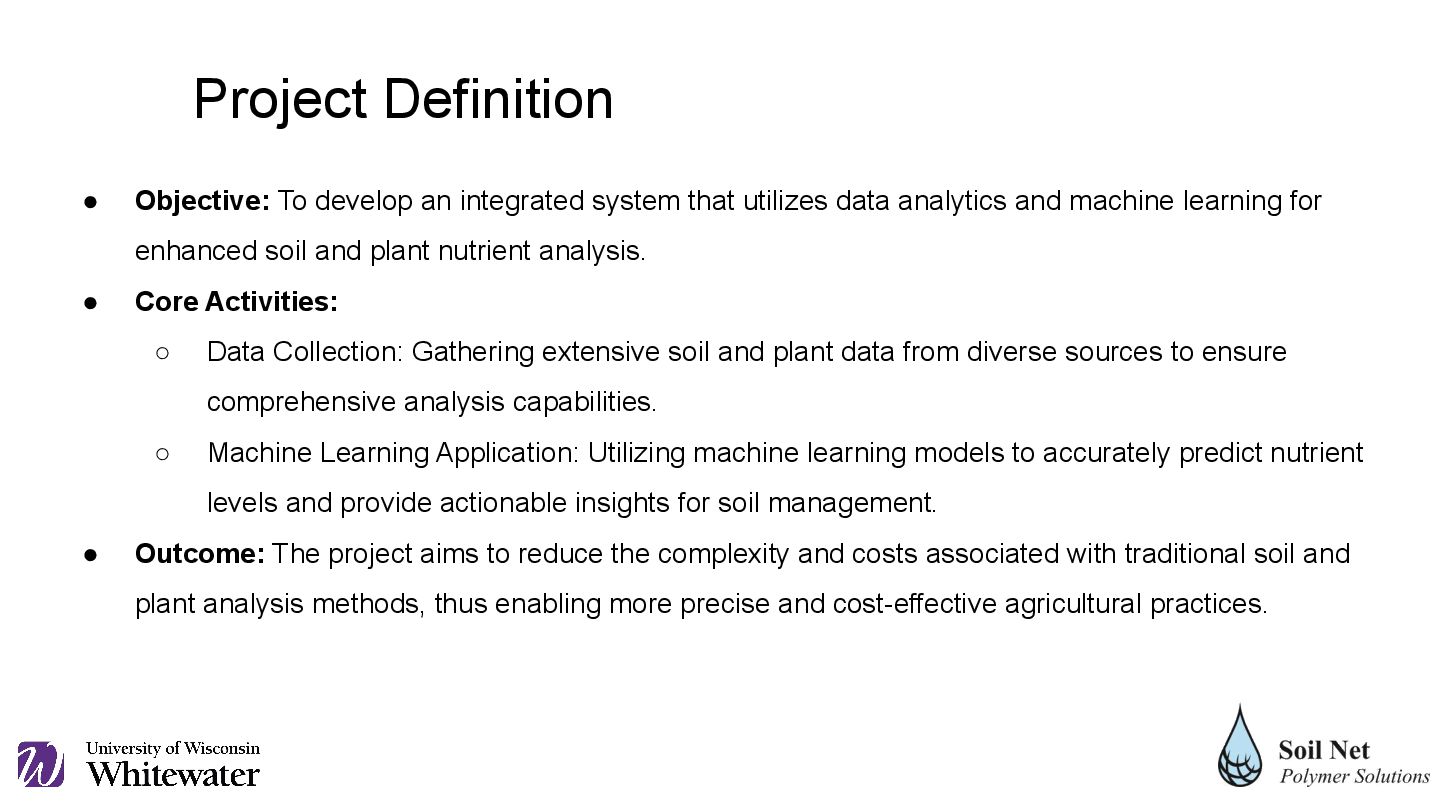
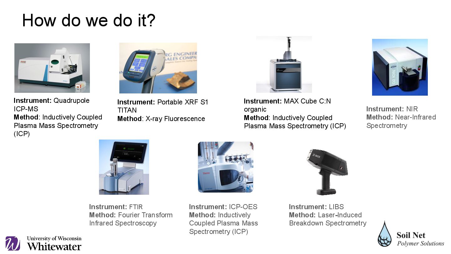
7. • Objective: To develop an integrated system that utilizes data analytics and machine learning for enhanced soil and plant nutrient analysis. • Core Activities: ◦ Data Collection: Gathering extensive soil and plant data from diverse sources to ensure comprehensive analysis capabilities. ◦ Machine Learning Application: Utilizing machine learning models to accurately predict nutrient levels and provide actionable insights for soil management. • Outcome: The project aims to reduce the complexity and costs associated with traditional soil and plant analysis methods, thus enabling more precise and cost-effective agricultural practices. Project Definition
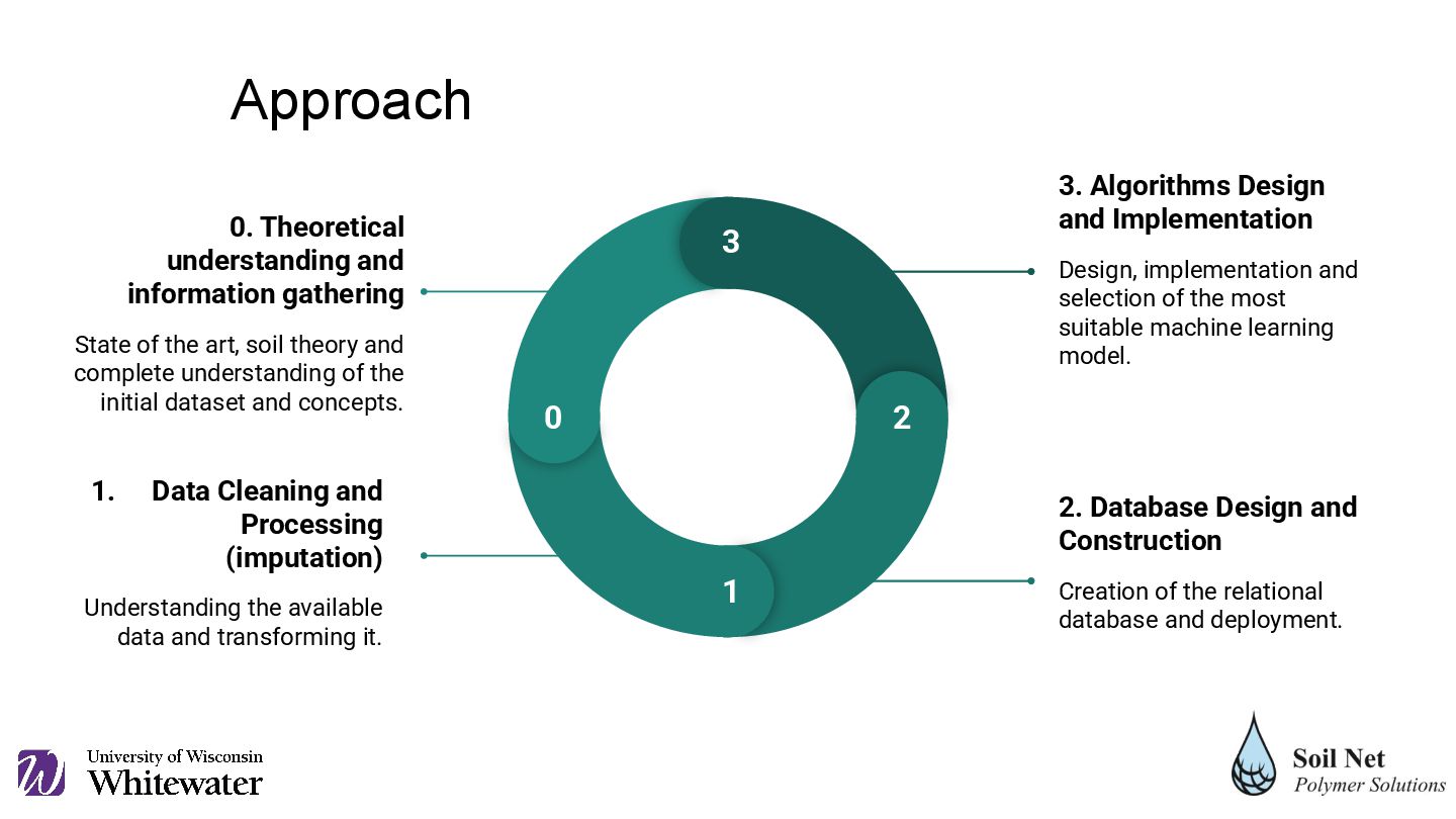
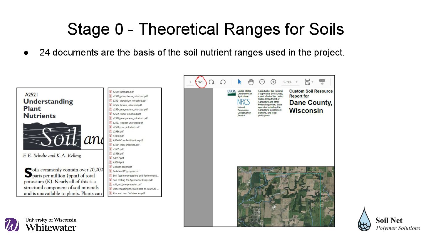
8. 1. Data Cleaning and Processing (imputation) Understanding the available data and transforming it. 2. Database Design and Construction Creation of the relational database and deployment. 3. Algorithms Design and Implementation Design, implementation and selection of the most suitable machine learning model. 0. Theoretical understanding and information gathering State of the art, soil theory and complete understanding of the initial dataset and concepts. 0 1 2 3 Approach
9. • 24 documents are the basis of the soil nutrient ranges used in the project. Stage 0 - Theoretical Ranges for Soils
10. How do we do it? Instrument: Quadrupole ICP-MS Method: Inductively Coupled Plasma Mass Spectrometry (ICP) Instrument: Portable XRF S1 TITAN Method: X-ray Fluorescence Instrument: MAX Cube C:N organic Method: Inductively Coupled Plasma Mass Spectrometry (ICP) Instrument: FTIR Method: Fourier Transform Infrared Spectroscopy Instrument: NIR Method: Near-Infrared Spectrometry Instrument: ICP-OES Method: Inductively Coupled Plasma Mass Spectrometry (ICP) Instrument: LIBS Method: Laser-Induced Breakdown Spectrometry
11. Initial Dataset Transformation
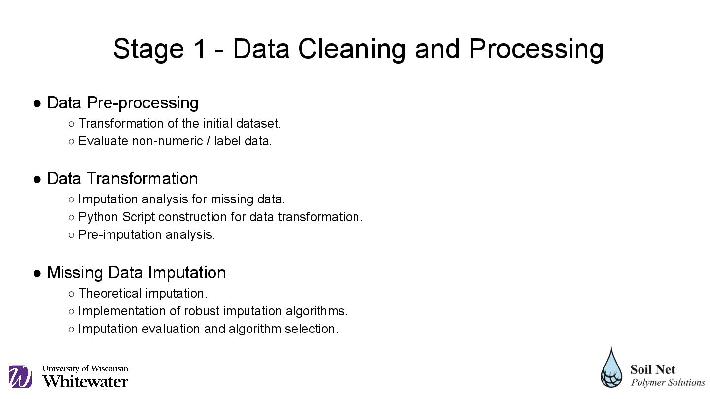
12. • Data Pre-processing ◦ Transformation of the initial dataset. ◦ Evaluate non-numeric / label data. • Data Transformation ◦ Imputation analysis for missing data. ◦ Python Script construction for data transformation. ◦ Pre-imputation analysis. • Missing Data Imputation ◦ Theoretical imputation. ◦ Implementation of robust imputation algorithms. ◦ Imputation evaluation and algorithm selection. Stage 1 - Data Cleaning and Processing
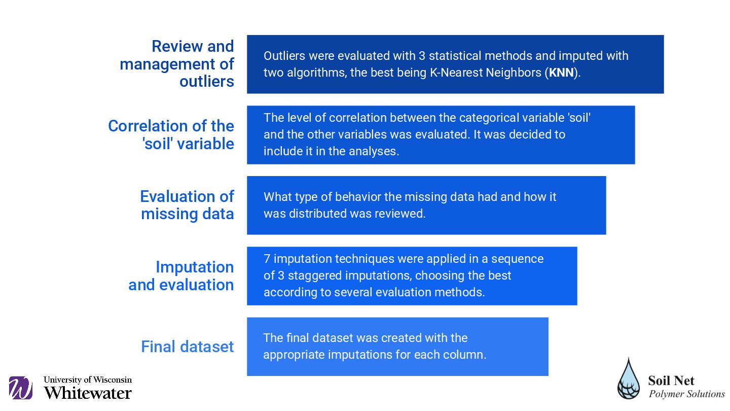
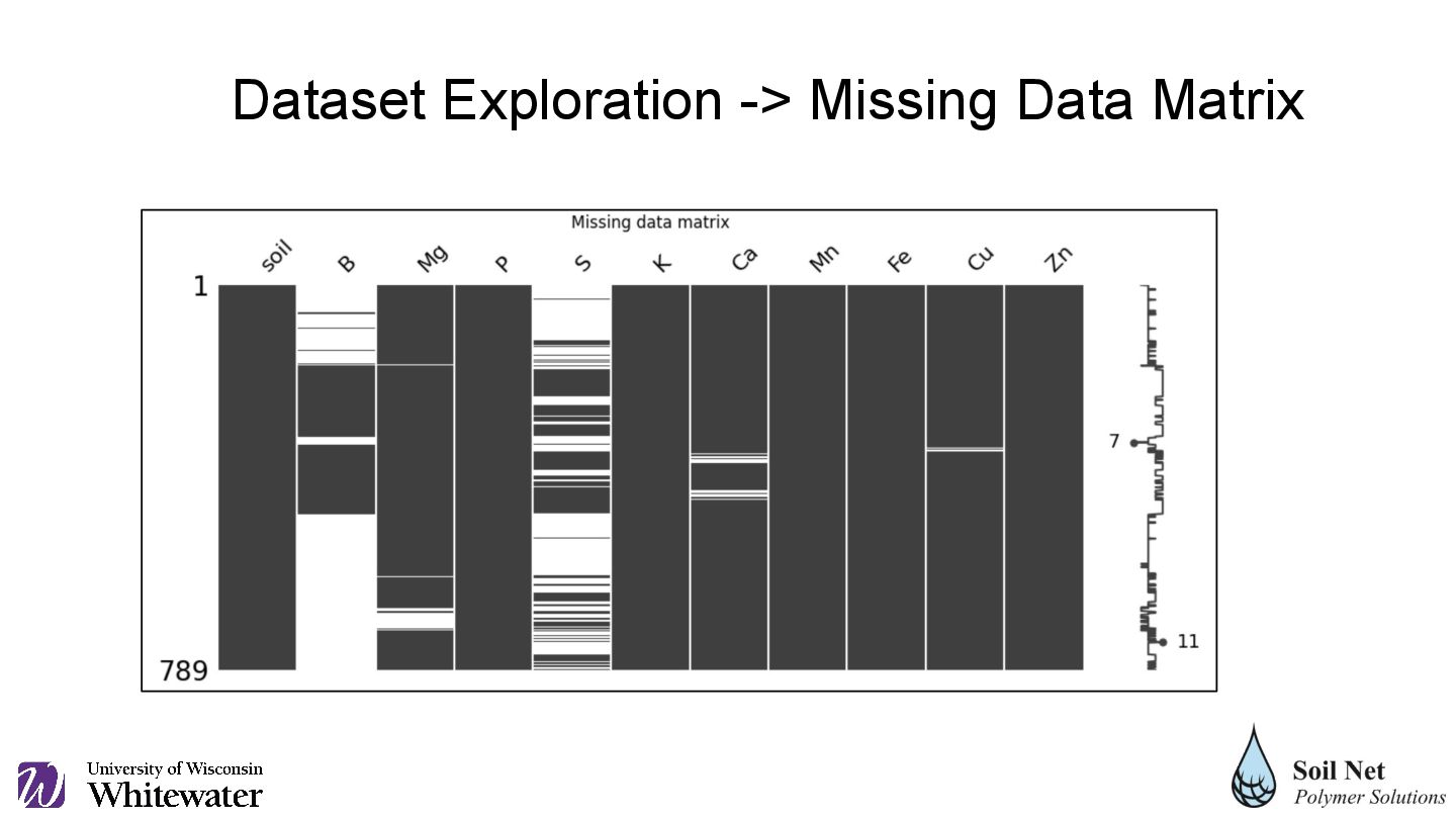
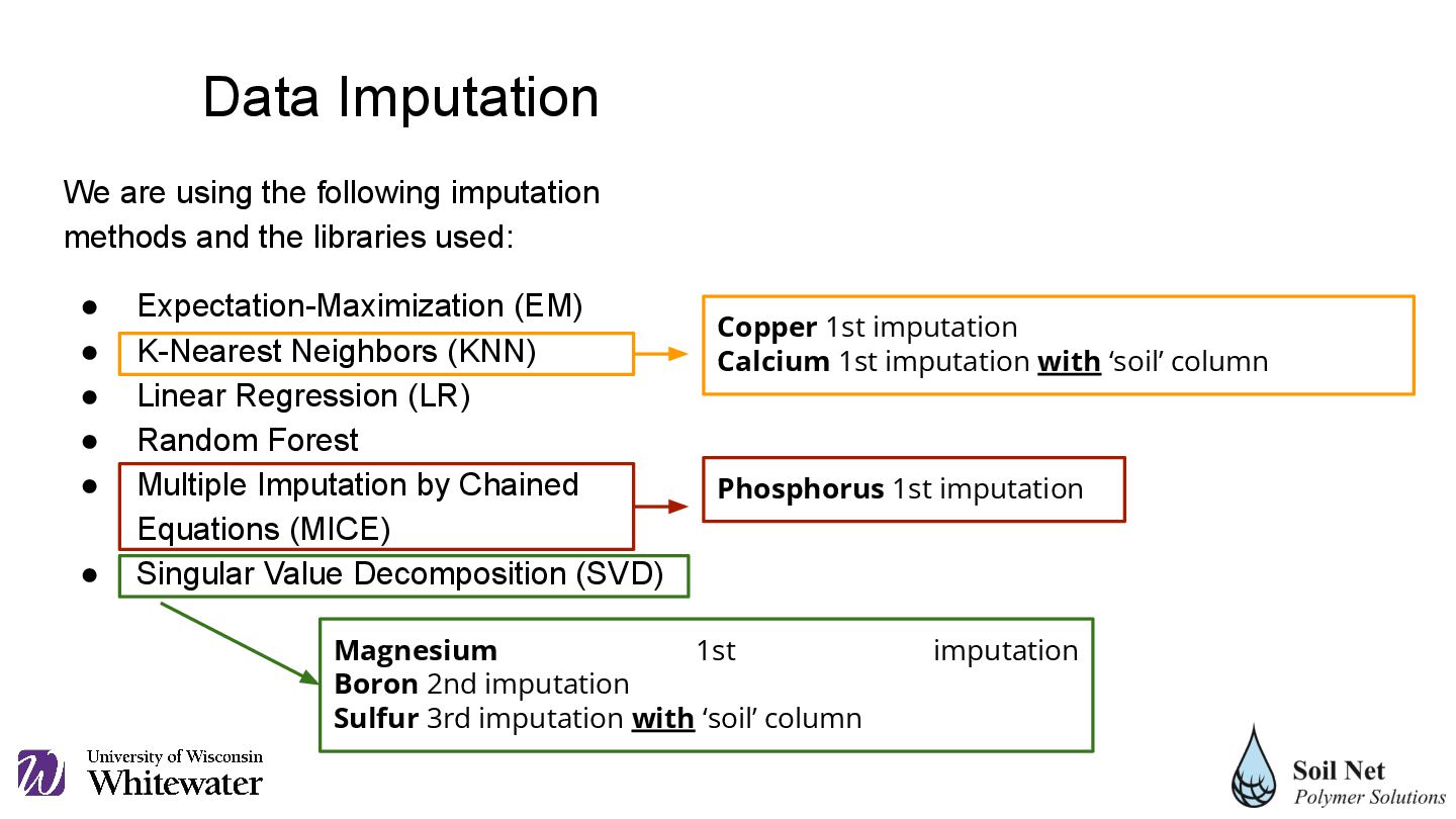
13. Review and management of outliers Outliers were evaluated with 3 statistical methods and imputed with two algorithms, the best being K-Nearest Neighbors (KNN). Correlation of the 'soil' variable The level of correlation between the categorical variable 'soil' and the other variables was evaluated. It was decided to include it in the analyses. Evaluation of missing data What type of behavior the missing data had and how it was distributed was reviewed. Imputation and evaluation 7 imputation techniques were applied in a sequence of 3 staggered imputations, choosing the best according to several evaluation methods. Final dataset The final dataset was created with the appropriate imputations for each column.
14. Librerías de Python (v3.11.x)
15. Otras herramientas (DevOps, DB and more)
16. Dataset Exploration - Distribution Analysis
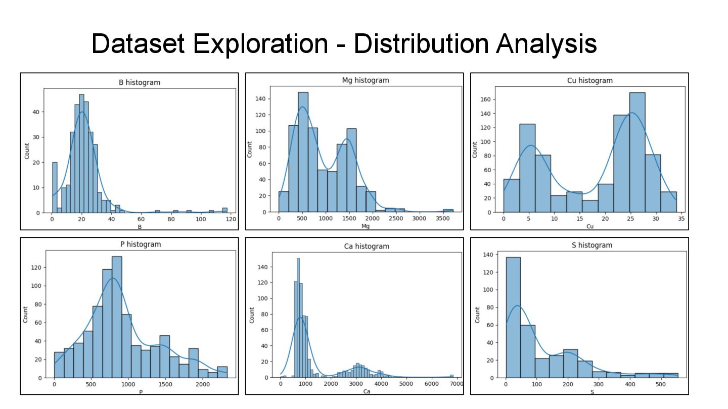
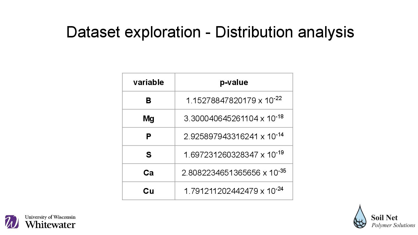
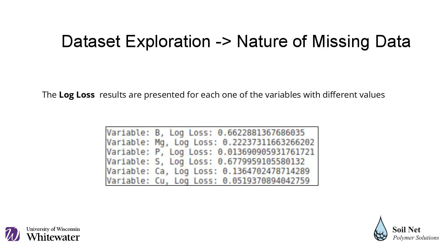
17. variable p-value B 1.15278847820179 x 10-22 Mg 3.300040645261104 x 10-18 P 2.925897943316241 x 10-14 S 1.697231260328347 x 10-19 Ca 2.8082234651365656 x 10-35 Cu 1.791211202442479 x 10-24 Dataset exploration - Distribution analysis
18. Dataset Exploration -> Missing Data Matrix
19. Boro (B) 62.36 % Azufre (S) 58.68 % Magnesio (Mg) 5.83 % Calcio (Ca) 3.04 % Cobre (Cu) 0.89 % Fósforo (P) 0.13 % Potasio (K) 0 % Manganeso (Mn) 0 % Hierro (Fe) 0 % Zinc (Zn) 0 % Soil Dataset Data Imputation: Step 2. Missing Data (%)
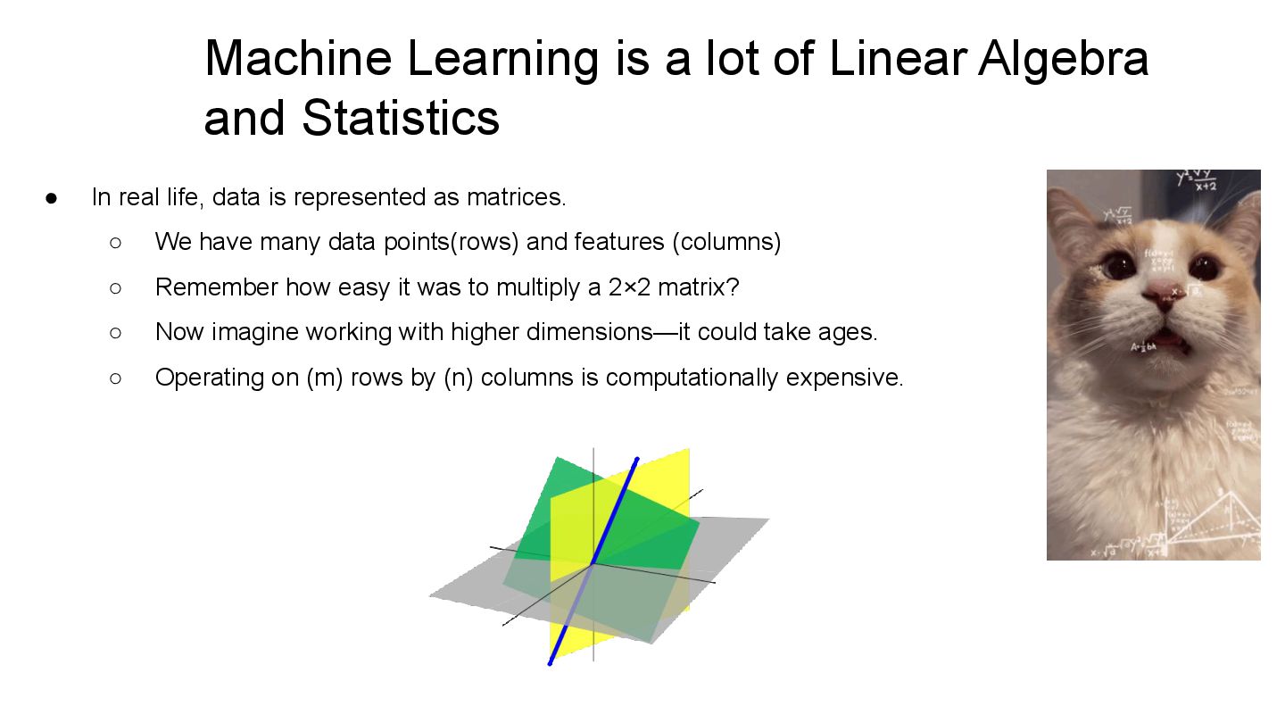
20. • In real life, data is represented as matrices. ◦ We have many data points(rows) and features (columns) ◦ Remember how easy it was to multiply a 2×2 matrix? ◦ Now imagine working with higher dimensions—it could take ages. ◦ Operating on (m) rows by (n) columns is computationally expensive. Machine Learning is a lot of Linear Algebra and Statistics
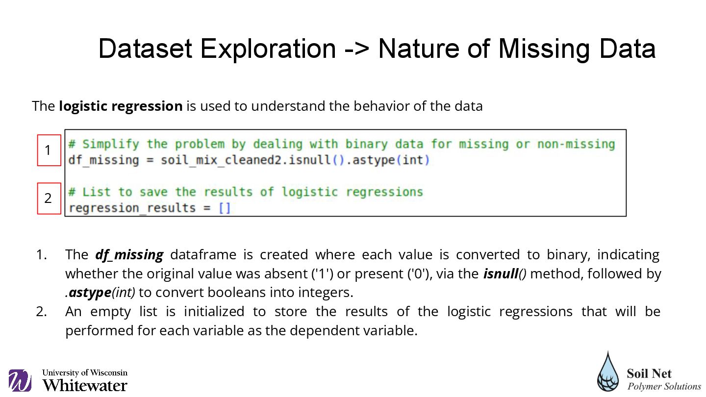
21. The logistic regression is used to understand the behavior of the data 1 2 1. The df_missing dataframe is created where each value is converted to binary, indicating whether the original value was absent ('1') or present ('0'), via the isnull() method, followed by .astype(int) to convert booleans into integers. 2. An empty list is initialized to store the results of the logistic regressions that will be performed for each variable as the dependent variable. Dataset Exploration -> Nature of Missing Data
22. The Log Loss results are presented for each one of the variables with different values Dataset Exploration -> Nature of Missing Data
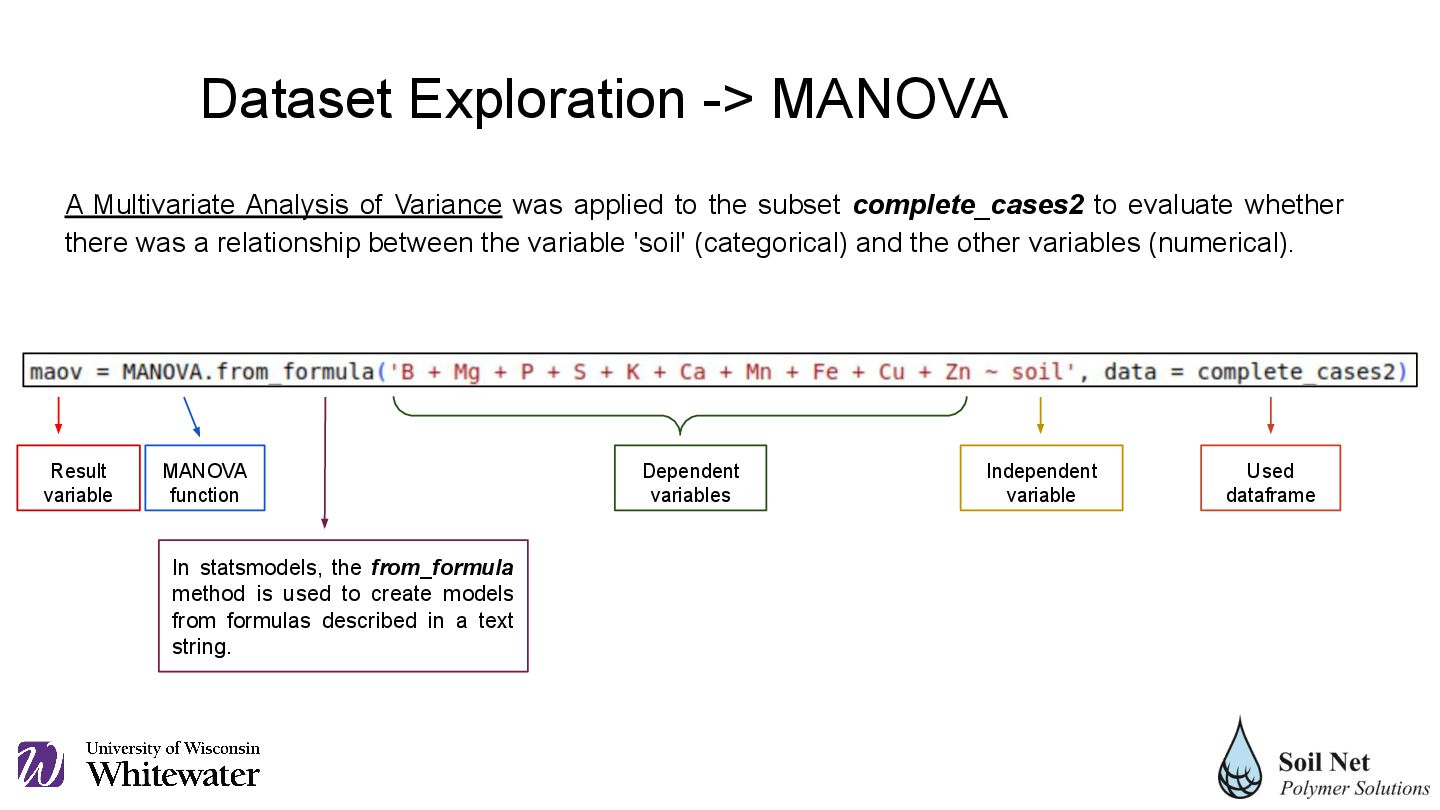
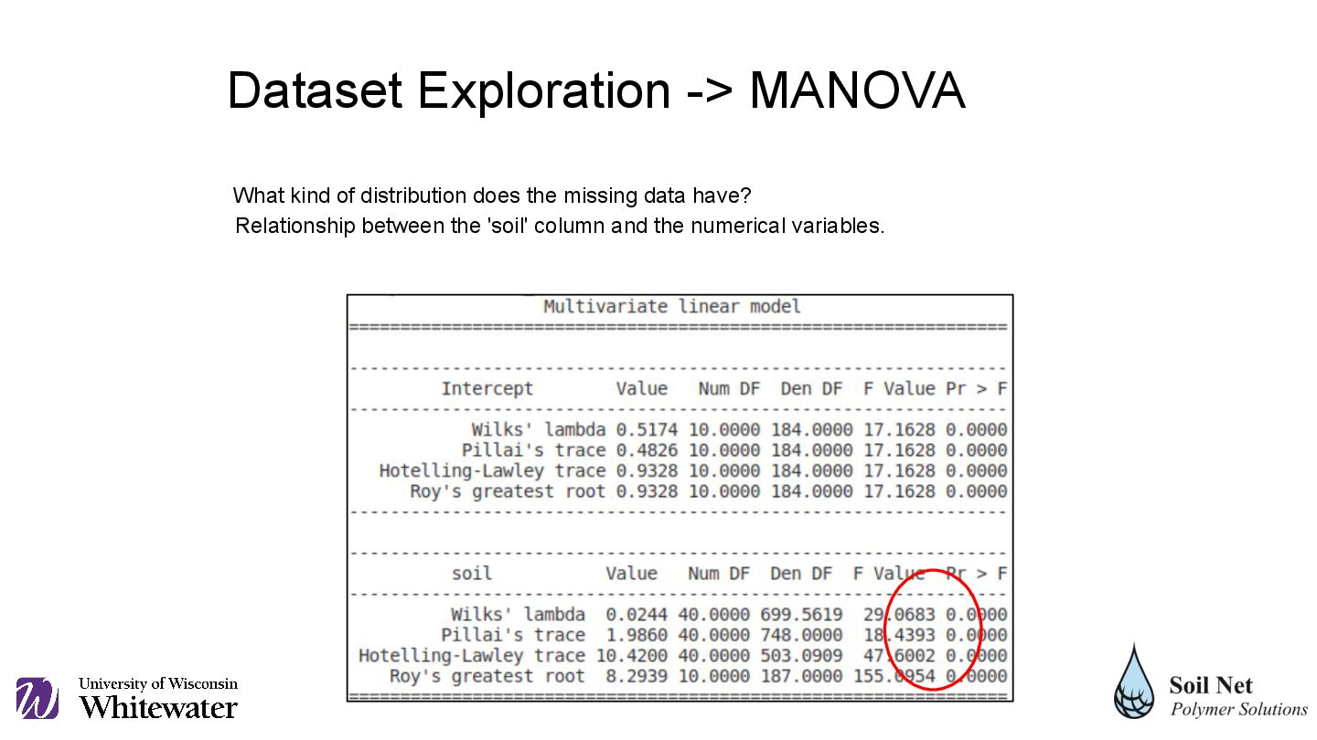
23. A Multivariate Analysis of Variance was applied to the subset complete_cases2 to evaluate whether there was a relationship between the variable 'soil' (categorical) and the other variables (numerical). Result variable MANOVA function In statsmodels, the from_formula method is used to create models from formulas described in a text string. Dependent variables Independent variable Used dataframe Dataset Exploration -> MANOVA
24. What kind of distribution does the missing data have? Relationship between the 'soil' column and the numerical variables. Dataset Exploration -> MANOVA
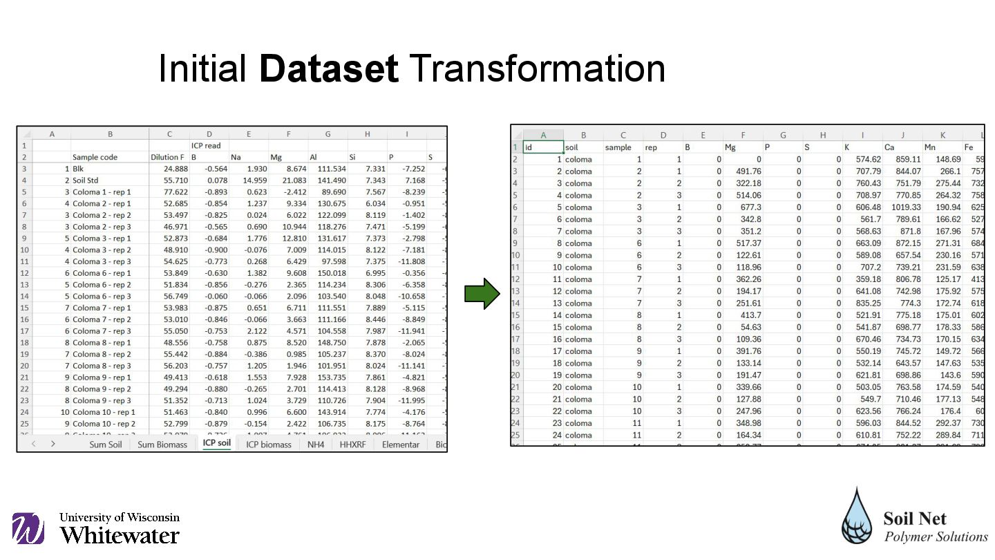
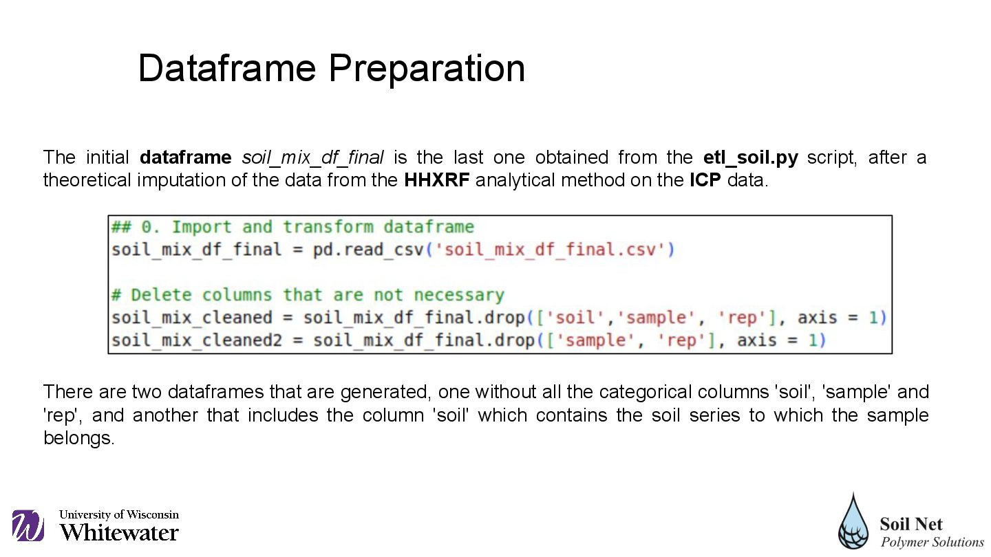
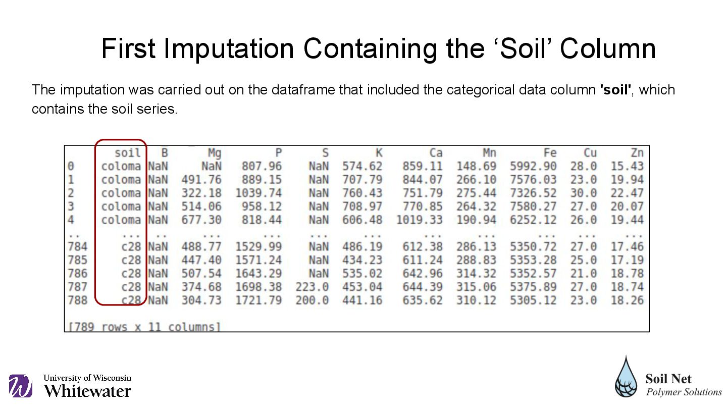
25. The initial dataframe soil_mix_df_final is the last one obtained from the etl_soil.py script, after a theoretical imputation of the data from the HHXRF analytical method on the ICP data. There are two dataframes that are generated, one without all the categorical columns 'soil', 'sample' and 'rep', and another that includes the column 'soil' which contains the soil series to which the sample belongs. Dataframe Preparation
26. We are using the following imputation methods and the libraries used: • Expectation-Maximization (EM) • K-Nearest Neighbors (KNN) • Linear Regression (LR) • Random Forest • Multiple Imputation by Chained Equations (MICE) • Singular Value Decomposition (SVD) Copper 1st imputation Calcium 1st imputation with ‘soil’ column Phosphorus 1st imputation Magnesium 1st imputation Boron 2nd imputation Sulfur 3rd imputation with ‘soil’ column Data Imputation
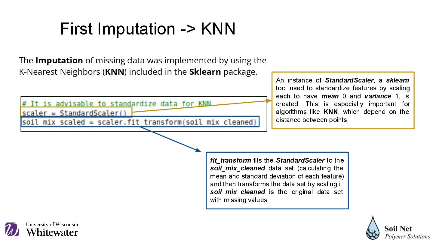
27. The Imputation of missing data was implemented by using the K-Nearest Neighbors (KNN) included in the Sklearn package. An instance of StandardScaler, a sklearn tool used to standardize features by scaling each to have mean 0 and variance 1, is created. This is especially important for algorithms like KNN, which depend on the distance between points; fit_transform fits the StandardScaler to the soil_mix_cleaned data set (calculating the mean and standard deviation of each feature) and then transforms the data set by scaling it. soil_mix_cleaned is the original data set with missing values. First Imputation -> KNN
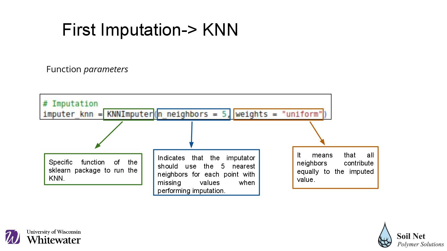
28. Specific function of the sklearn package to run the KNN. Indicates that the imputator should use the 5 nearest neighbors for each point with missing values when performing imputation. It means that all neighbors contribute equally to the imputed value. Function parameters First Imputation-> KNN
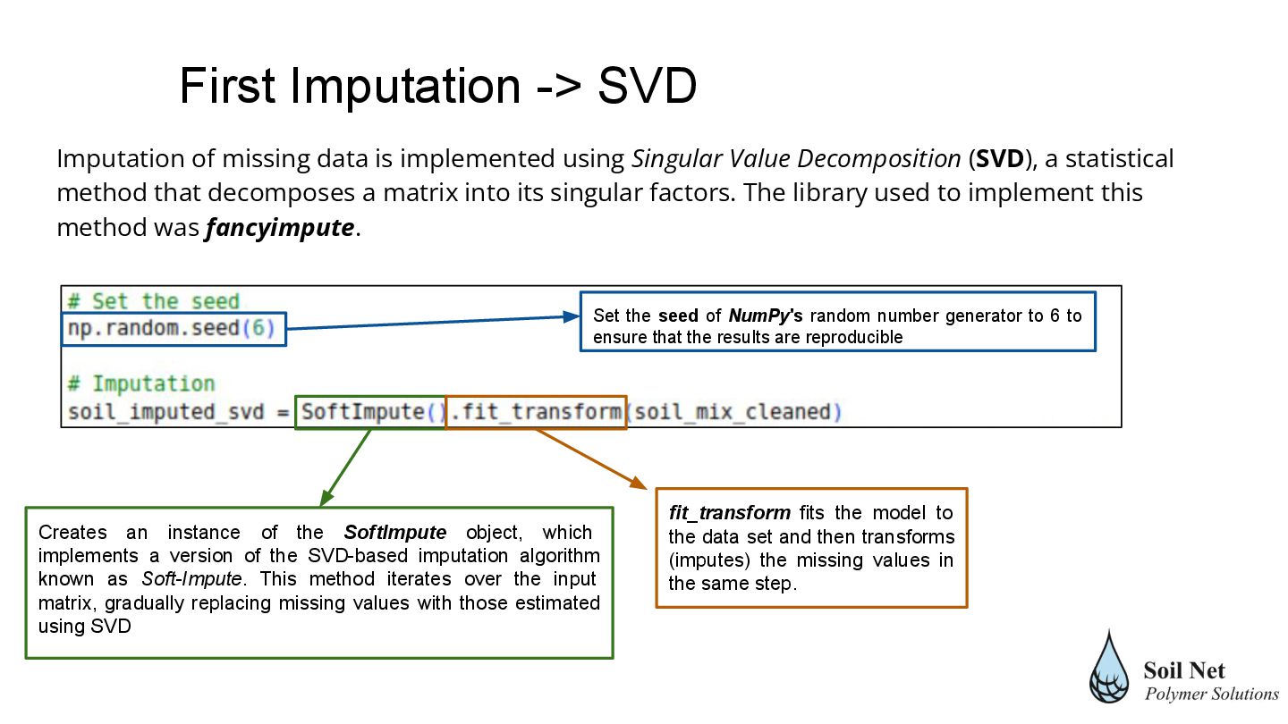
29. Imputation of missing data is implemented using Singular Value Decomposition (SVD), a statistical method that decomposes a matrix into its singular factors. The library used to implement this method was fancyimpute. Creates an instance of the SoftImpute object, which implements a version of the SVD-based imputation algorithm known as Soft-Impute. This method iterates over the input matrix, gradually replacing missing values with those estimated using SVD Set the seed of NumPy's random number generator to 6 to ensure that the results are reproducible fit_transform fits the model to the data set and then transforms (imputes) the missing values in the same step. First Imputation -> SVD
30. The imputation was carried out on the dataframe that included the categorical data column 'soil', which contains the soil series. First Imputation Containing the ‘Soil’ Column
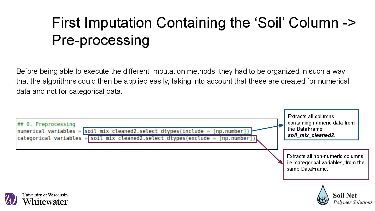
31. Before being able to execute the different imputation methods, they had to be organized in such a way that the algorithms could then be applied easily, taking into account that these are created for numerical data and not for categorical data. Extracts all columns containing numeric data from the DataFrame soil_mix_cleaned2. Extracts all non-numeric columns, i.e. categorical variables, from the same DataFrame. First Imputation Containing the ‘Soil’ Column -> Pre-processing
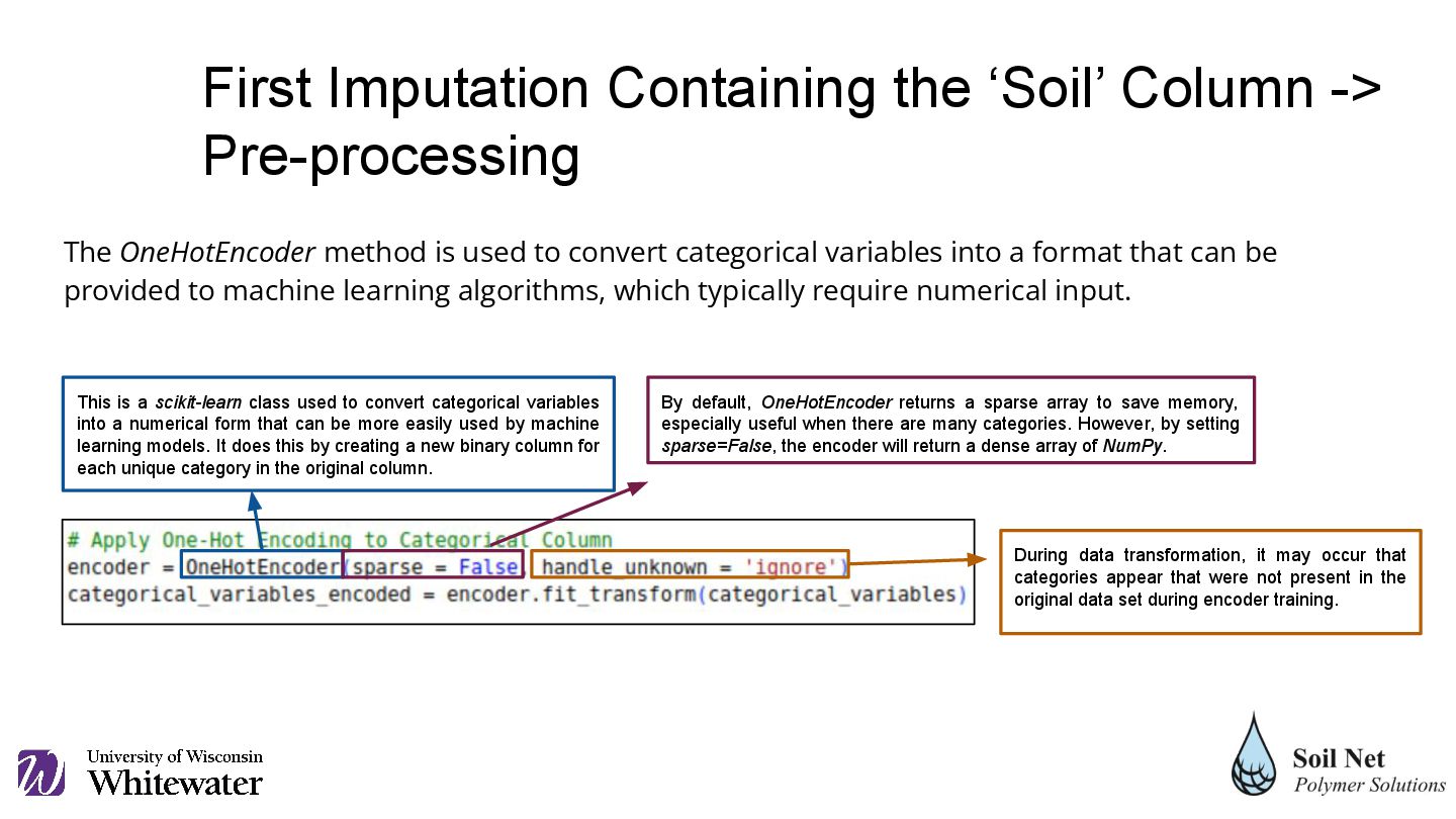
32. The OneHotEncoder method is used to convert categorical variables into a format that can be provided to machine learning algorithms, which typically require numerical input. This is a scikit-learn class used to convert categorical variables into a numerical form that can be more easily used by machine learning models. It does this by creating a new binary column for each unique category in the original column. During data transformation, it may occur that categories appear that were not present in the original data set during encoder training. By default, OneHotEncoder returns a sparse array to save memory, especially useful when there are many categories. However, by setting sparse=False, the encoder will return a dense array of NumPy. First Imputation Containing the ‘Soil’ Column -> Pre-processing
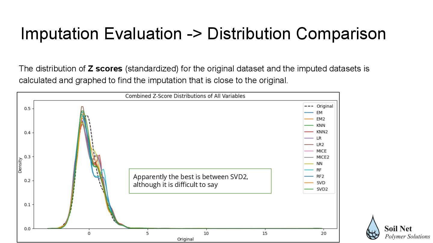
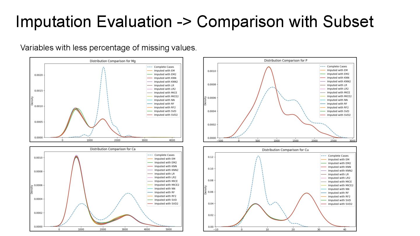
33. The distribution of Z scores (standardized) for the original dataset and the imputed datasets is calculated and graphed to find the imputation that is close to the original. Apparently the best is between SVD2, although it is difficult to say Imputation Evaluation -> Distribution Comparison
34. Imputation Evaluation -> Correlation Analysis
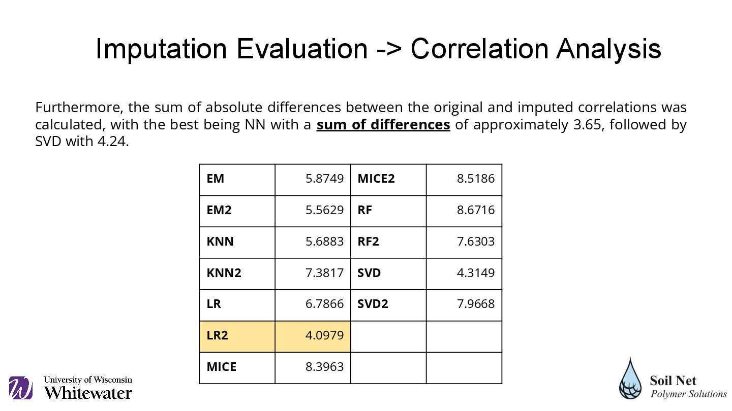
35. Furthermore, the sum of absolute differences between the original and imputed correlations was calculated, with the best being NN with a sum of differences of approximately 3.65, followed by SVD with 4.24. EM 5.8749 MICE2 8.5186 EM2 5.5629 RF 8.6716 KNN 5.6883 RF2 7.6303 KNN2 7.3817 SVD 4.3149 LR 6.7866 SVD2 7.9668 LR2 4.0979 MICE 8.3963 Imputation Evaluation -> Correlation Analysis
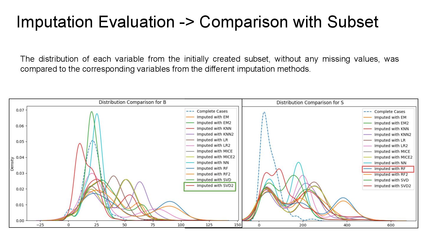
36. The distribution of each variable from the initially created subset, without any missing values, was compared to the corresponding variables from the different imputation methods. Imputation Evaluation -> Comparison with Subset
37. Variables with less percentage of missing values. Imputation Evaluation -> Comparison with Subset
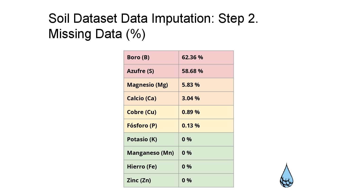
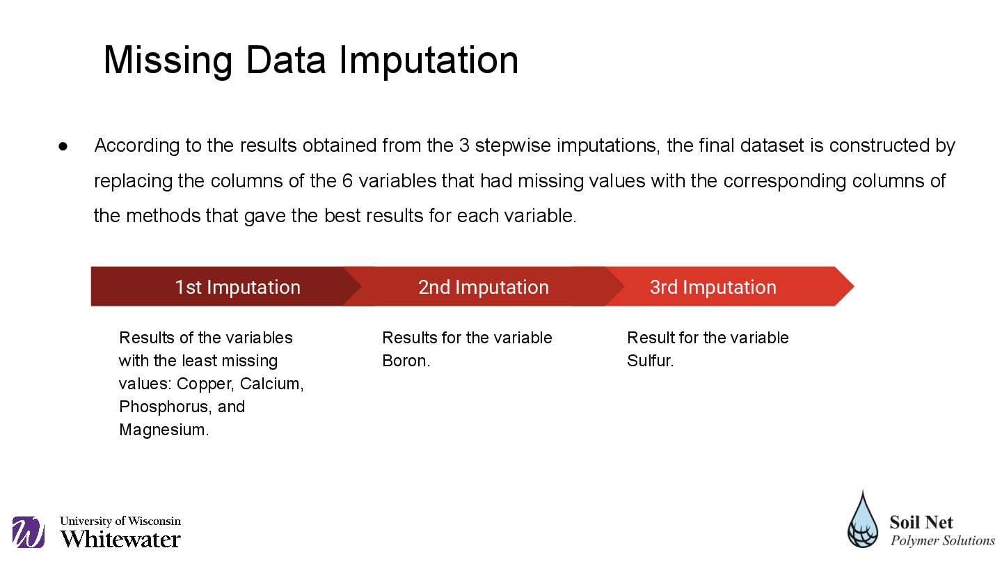
38. • According to the results obtained from the 3 stepwise imputations, the final dataset is constructed by replacing the columns of the 6 variables that had missing values with the corresponding columns of the methods that gave the best results for each variable. 3rd Imputation Result for the variable Sulfur. 1st Imputation Results of the variables with the least missing values: Copper, Calcium, Phosphorus, and Magnesium. 2nd Imputation Results for the variable Boron. Missing Data Imputation
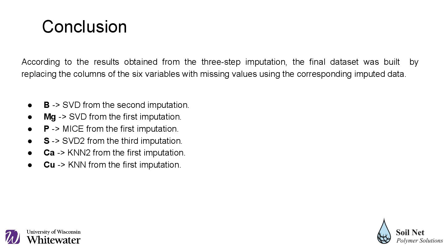
39. Conclusion According to the results obtained from the three-step imputation, the final dataset was built by replacing the columns of the six variables with missing values using the corresponding imputed data. • B -> SVD from the second imputation. • Mg -> SVD from the first imputation. • P -> MICE from the first imputation. • S -> SVD2 from the third imputation. • Ca -> KNN2 from the first imputation. • Cu -> KNN from the first imputation.
40. https://www.researchgate.net/publication/322179244_Data_Mining_Accuracy_and_Error_Measure s_for_Classification_and_Prediction Phase 3 - Bootstrapping for Dataset size augmentation
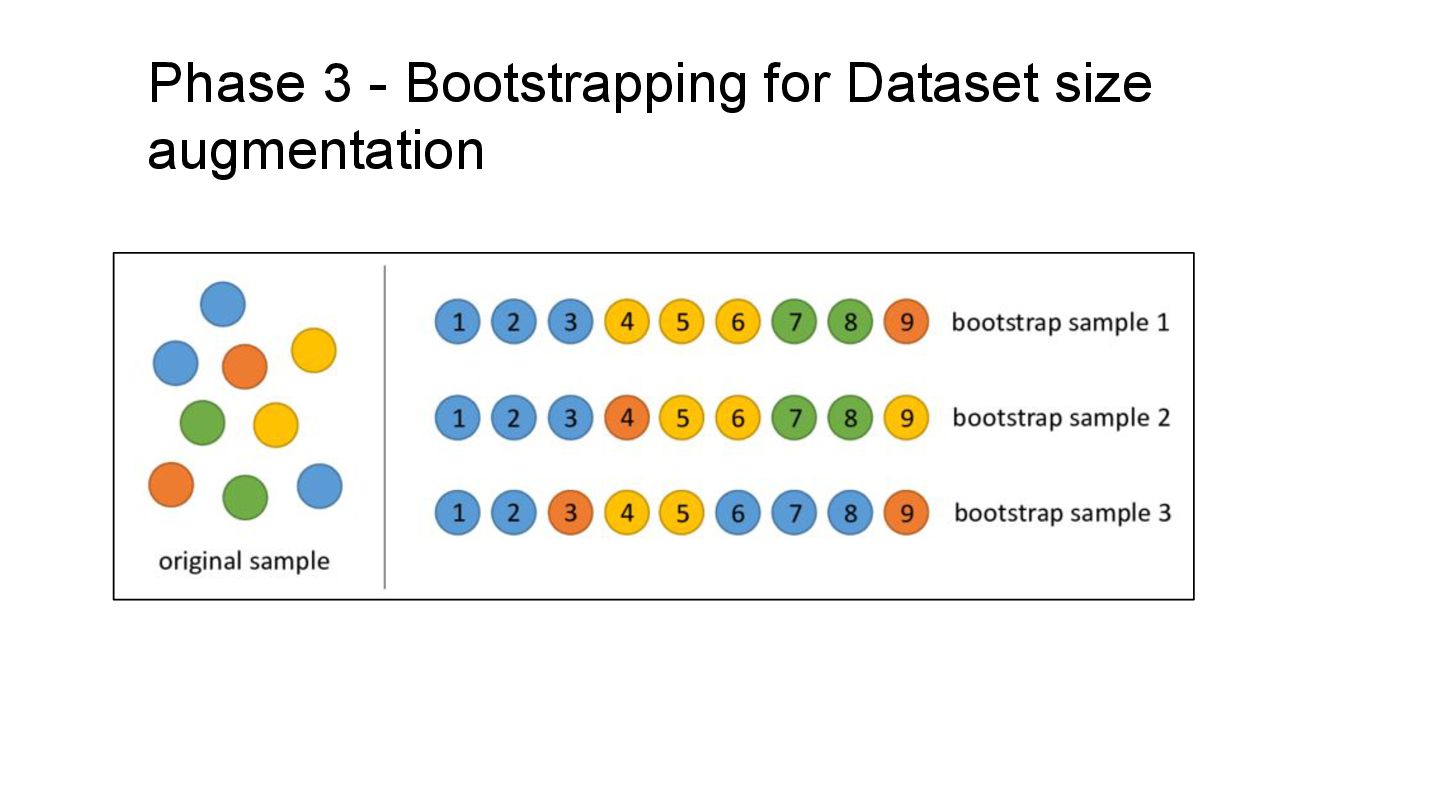
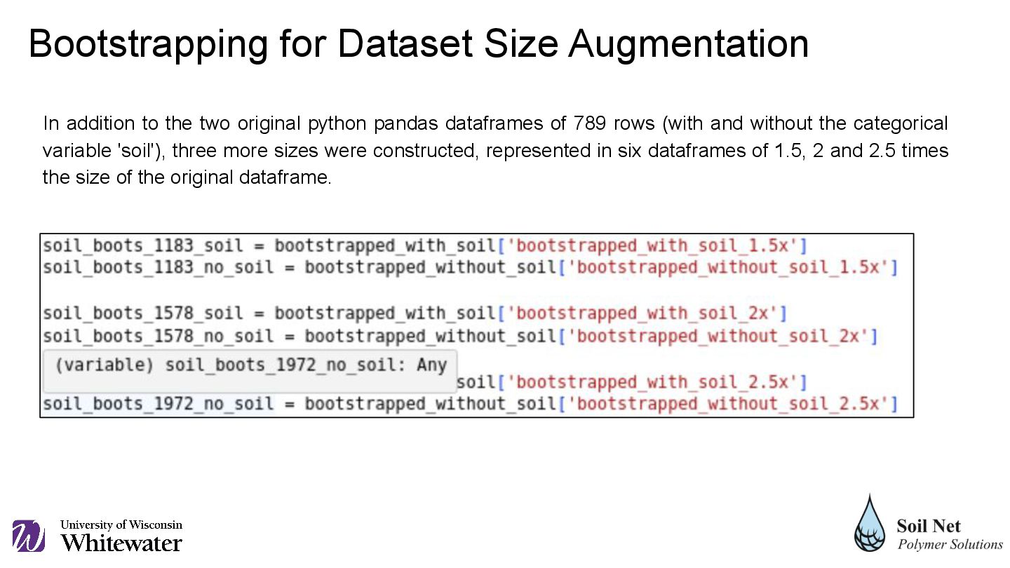
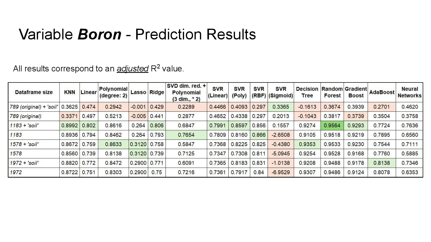
41. Bootstrapping for Dataset Size Augmentation In addition to the two original python pandas dataframes of 789 rows (with and without the categorical variable 'soil'), three more sizes were constructed, represented in six dataframes of 1.5, 2 and 2.5 times the size of the original dataframe.
42. Bootstrapping Evaluation
43. Bootstrapping Evaluation - Density Distribution
44. Machine Learning Models Implemented • K-Nearest Neighbors (KNN) • Linear Regression • Polynomial Regression • Lasso Regression • Ridge Regression • Singular Value Decomposition to reduce dimensionality • Support Vector Regression (SVR) • Decision Trees • Random Forest • Gradient Boost • AdaBoost
45. Variable Boron - Prediction Results All results correspond to an adjusted R2 value.
46. Random Forest Regressor – N N - Mean MSE: 0.0250 Std MSE: 0.0129 MAE: 0.0282 MSE: 0.0032 R2: 0.9870 MAPE: 0.95%
47. Random Forest Regressor – P P - Mean MSE: 291165.2807 Std MSE: 156837.0345 MAE: 102.8173 MSE: 37130.9636 R2: 0.9435 MAPE: 3.19%
48. Random Forest Regressor – K K - Mean MSE: 14722715.9774 Std MSE: 4476349.2071 MAE: 812.6680 MSE: 2130879.6496 R2: 0.9753 MAPE: 2.87%
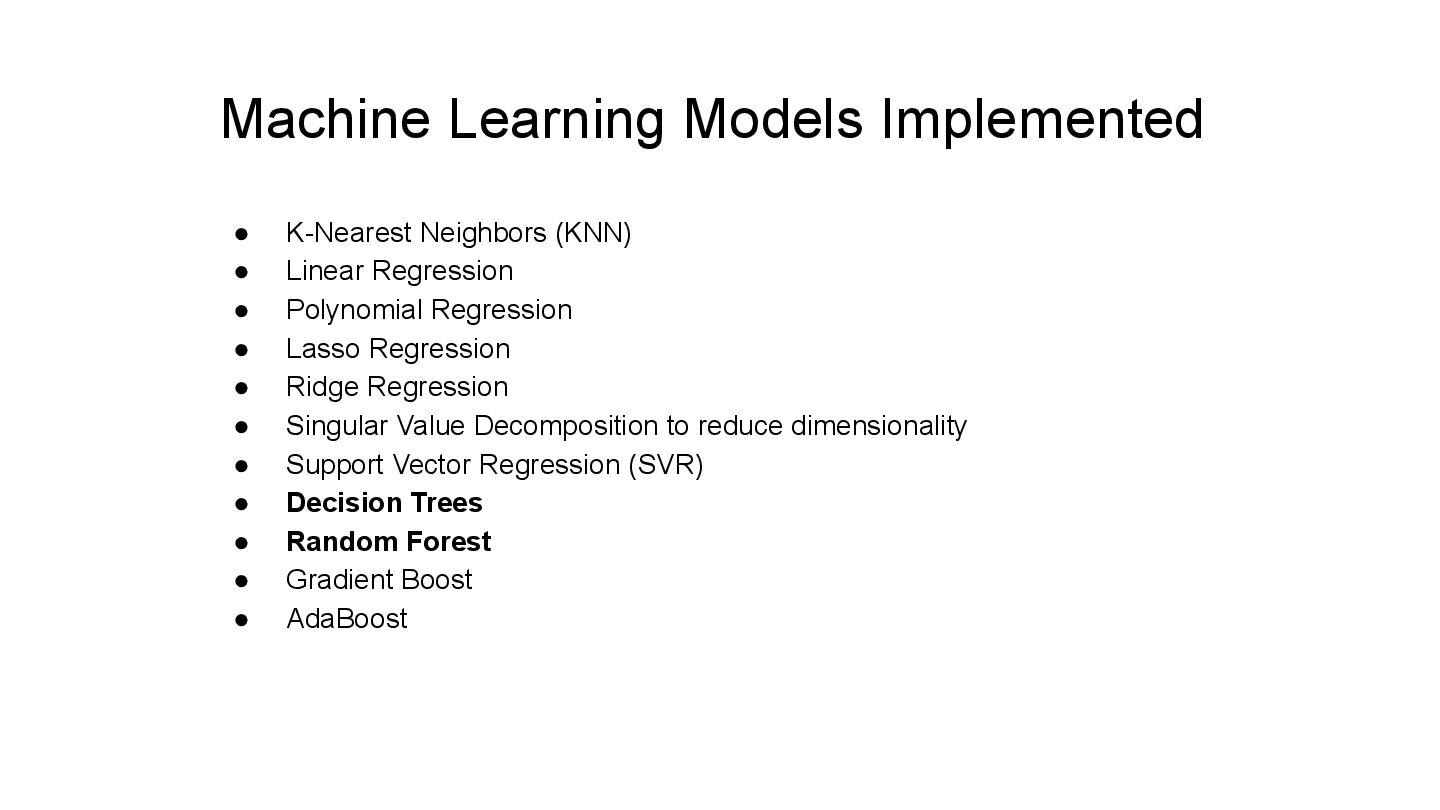
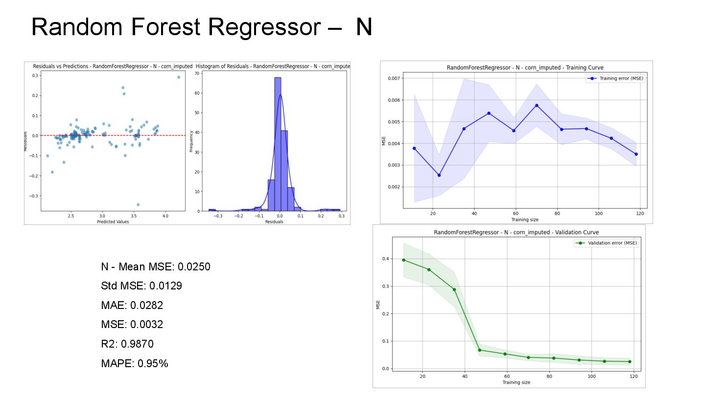
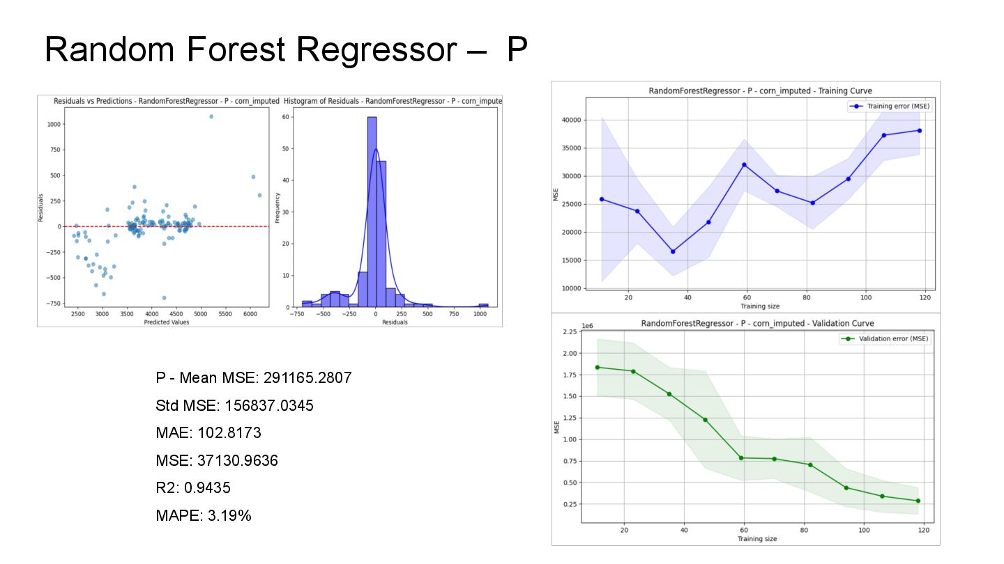
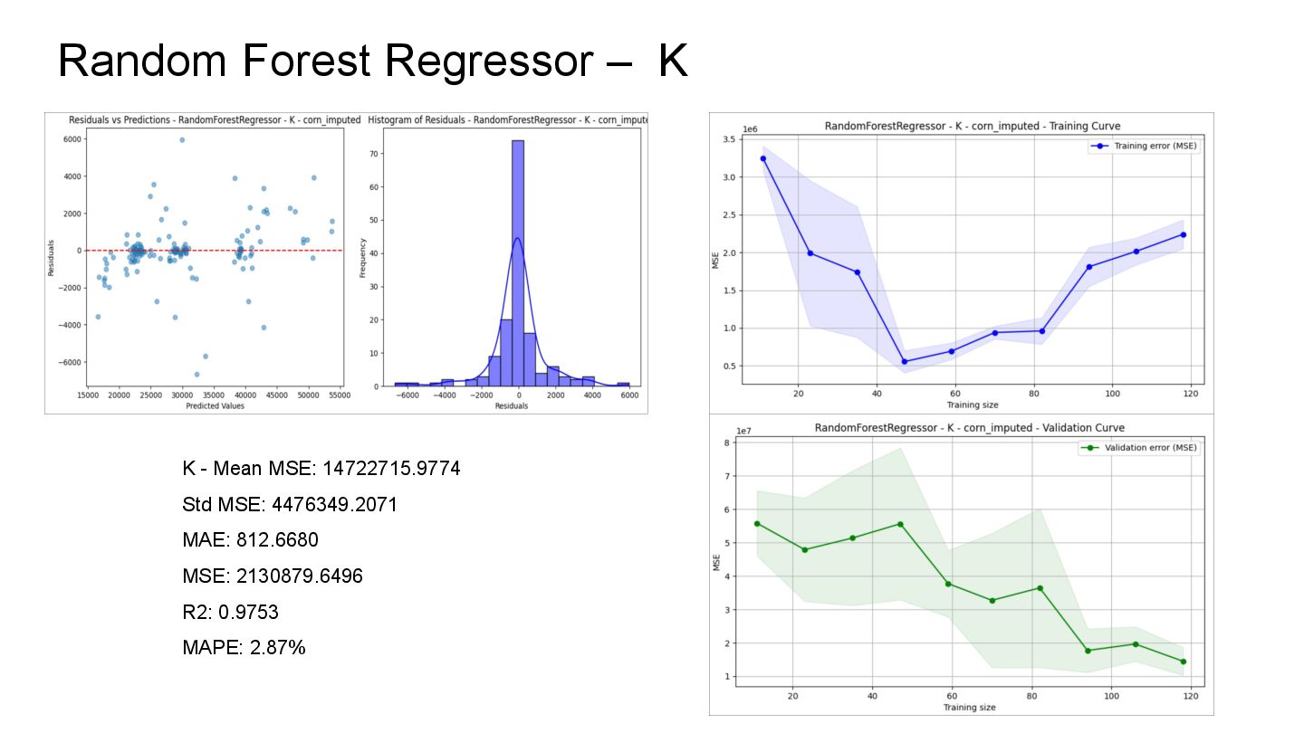
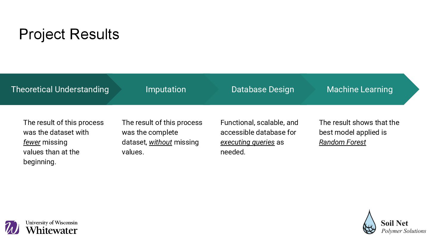
49. Project Results Theoretical Understanding The result of this process was the dataset with fewer missing values than at the beginning. Imputation The result of this process was the complete dataset, without missing values. Database Design Functional, scalable, and accessible database for executing queries as needed. Machine Learning The result shows that the best model applied is Random Forest
50. Open source research available on Kaggle Data Imputation with ML: https://www.kaggle.com/code/juandavidroavalencia/data-imputation Outliers Review: https://www.kaggle.com/code/juandavidroavalencia/outliers-review Soils ETL: https://www.kaggle.com/code/juandavidroavalencia/soils-etl