can you answer these questions? What does the t-test do? Ways you can answer the question i.e. communicate your understanding: Explain the test verbally Perform the data analysis
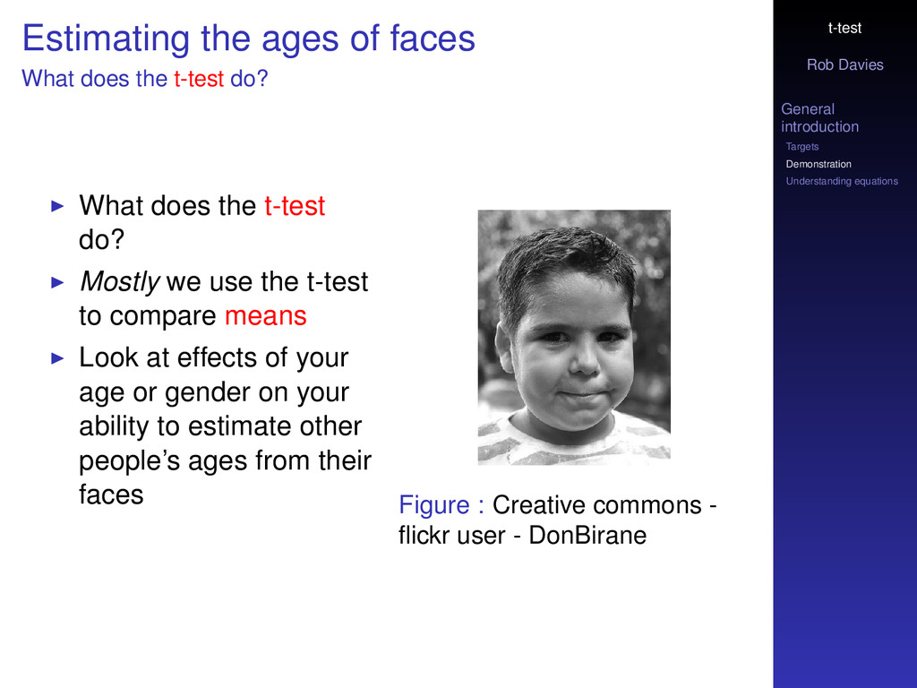
the ages of faces What does the t-test do? What does the t-test do? Mostly we use the t-test to compare means Look at effects of your age or gender on your ability to estimate other people’s ages from their faces Figure : Creative commons - flickr user - DonBirane
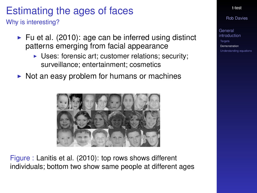
the ages of faces Why is interesting? Fu et al. (2010): age can be inferred using distinct patterns emerging from facial appearance Uses: forensic art; customer relations; security; surveillance; entertainment; cosmetics Not an easy problem for humans or machines Figure : Lanitis et al. (2010): top rows shows different individuals; bottom two show same people at different ages
your task is to estimate the age of each of six people Voelkle et al. (2011) asked young, middle-aged and older adults of both genders to estimate the ages of people whose faces were shown. Older and young adults, were more accurate and less biased in estimating the age of members of their own as compared with those of the other age group No reliable own-gender advantage was observed We can test the hypothesis: People—you—are more accurate in estimating the age of other people your own age
does the t-test do? Key vocabulary We can express our understanding of the t-test and what we do with it verbally Mostly we use the t-test to compare sample means What does this signify?
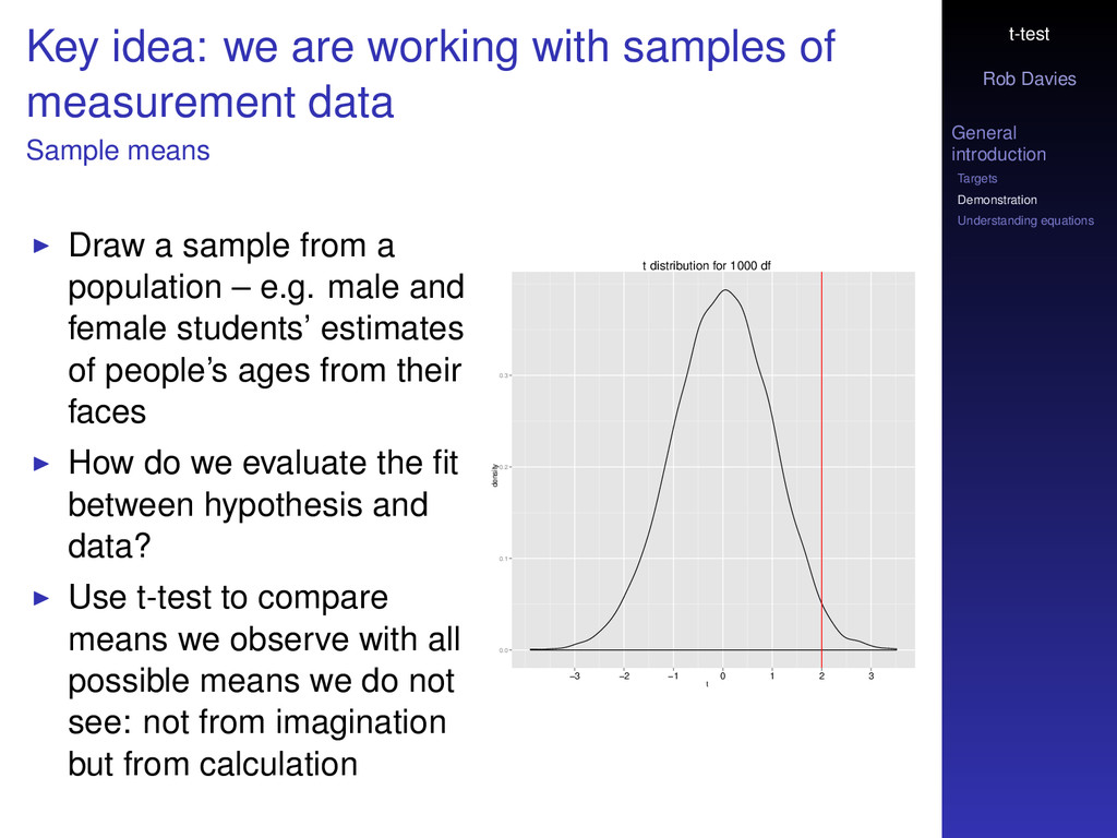
idea: we are working with samples of measurement data Sample means Draw a sample from a population – e.g. male and female students’ estimates of people’s ages from their faces How do we evaluate the fit between hypothesis and data? Use t-test to compare means we observe with all possible means we do not see: not from imagination but from calculation t distribution for 1000 df t density 0.0 0.1 0.2 0.3 −3 −2 −1 0 1 2 3
means The research and the null hypothesis We care about our question: is age estimation more accurate if faces are from the same age group? We answer the question using Null Hypothesis Significance Testing What is the null hypothesis here? No difference between errors to same or different aged people Why do we do this? We compare what we observe with what we would observe if the null hypothesis were true It is easier to calculate what potential values for a statistic would like if nothing was happening except random variation
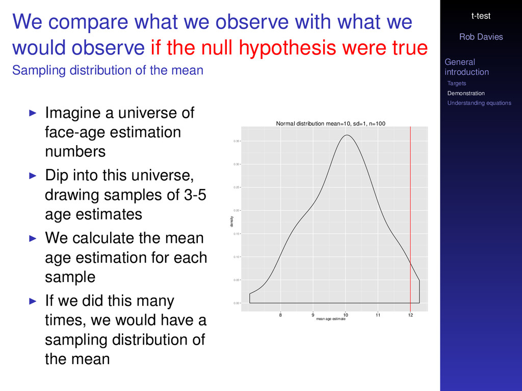
compare what we observe with what we would observe if the null hypothesis were true Sampling distribution of the mean Imagine a universe of face-age estimation numbers Dip into this universe, drawing samples of 3-5 age estimates We calculate the mean age estimation for each sample If we did this many times, we would have a sampling distribution of the mean Normal distribution mean=10, sd=1, n=100 mean age estimate density 0.00 0.05 0.10 0.15 0.20 0.25 0.30 0.35 8 9 10 11 12
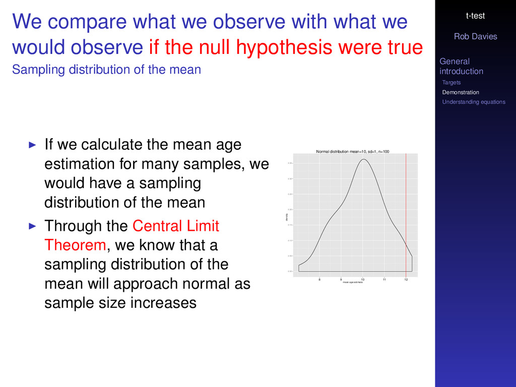
compare what we observe with what we would observe if the null hypothesis were true Sampling distribution of the mean If we calculate the mean age estimation for many samples, we would have a sampling distribution of the mean Through the Central Limit Theorem, we know that a sampling distribution of the mean will approach normal as sample size increases Normal distribution mean=10, sd=1, n=100 mean age estimate density 0.00 0.05 0.10 0.15 0.20 0.25 0.30 0.35 8 9 10 11 12
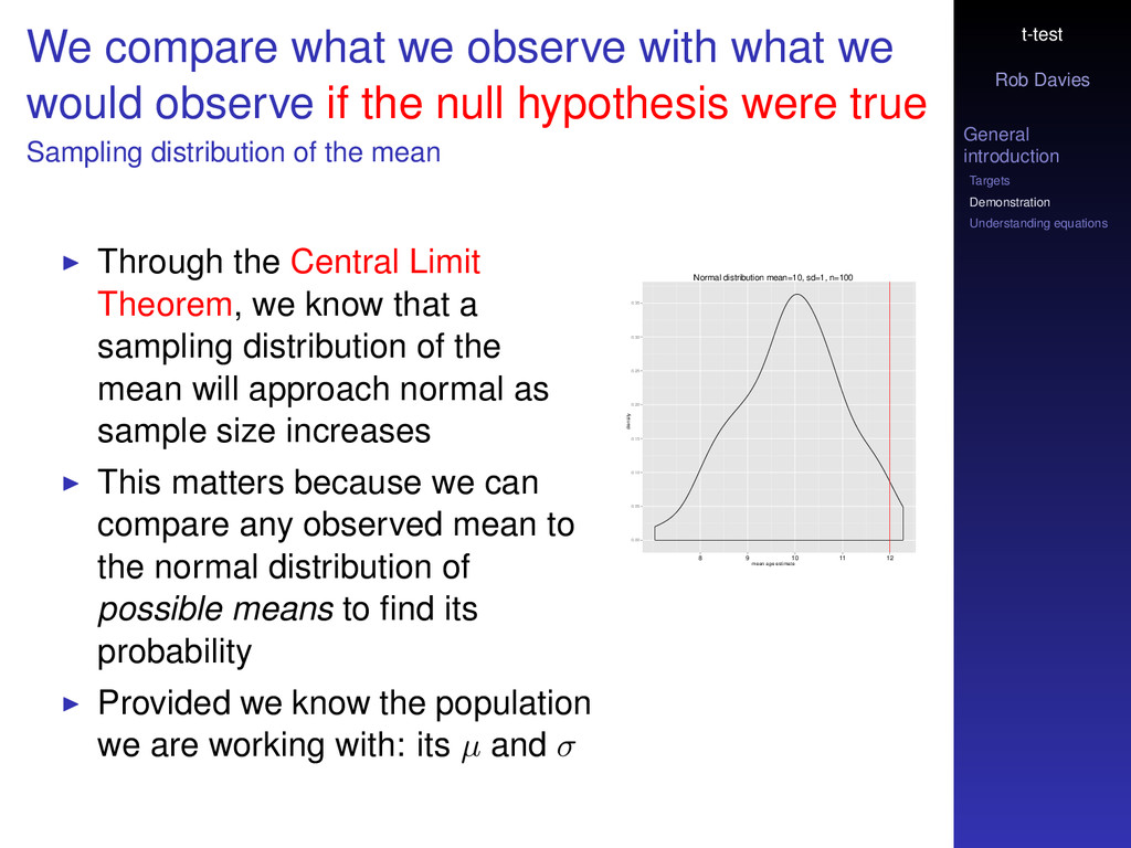
compare what we observe with what we would observe if the null hypothesis were true Sampling distribution of the mean Through the Central Limit Theorem, we know that a sampling distribution of the mean will approach normal as sample size increases This matters because we can compare any observed mean to the normal distribution of possible means to find its probability Provided we know the population we are working with: its µ and σ Normal distribution mean=10, sd=1, n=100 mean age estimate density 0.00 0.05 0.10 0.15 0.20 0.25 0.30 0.35 8 9 10 11 12
vocabulary Central Limit Theorem, CLT Central Limit Theorem [short version]: the sampling distribution of the mean approaches normal as n increases Central Limit Theorem [long version]: Given a population with mean µ and variance σ2 . . . the sampling distribution of the mean will have a mean equal to mu, a variance equal to σ2 divided by n, and a standard deviation equal to sigma over root n. The distribution will approach normal as n, the sample size increases.
vocabulary Central Limit Theorem, CLT Central Limit Theorem [short version]: the sampling distribution of the mean approaches normal as n increases What does this signify? It tells us what the mean and variance of the sampling distribution of the mean must be for any given sample size It also states that as n increases, the shape of this sampling distribution approaches normal, whatever the shape of the parent population.
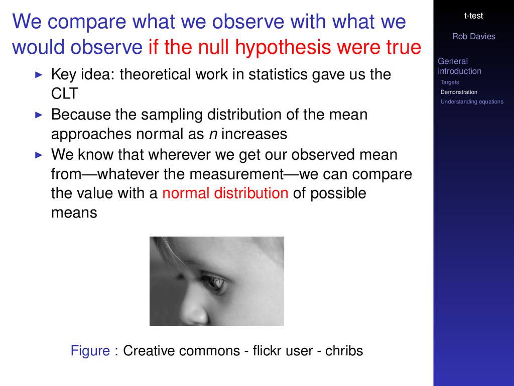
compare what we observe with what we would observe if the null hypothesis were true Key idea: theoretical work in statistics gave us the CLT Because the sampling distribution of the mean approaches normal as n increases We know that wherever we get our observed mean from—whatever the measurement—we can compare the value with a normal distribution of possible means Figure : Creative commons - flickr user - chribs
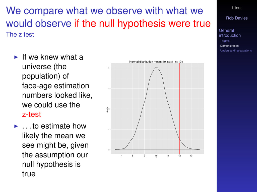
compare what we observe with what we would observe if the null hypothesis were true The z test If we knew what a universe (the population) of face-age estimation numbers looked like, we could use the z-test . . . to estimate how likely the mean we see might be, given the assumption our null hypothesis is true Normal distribution mean=10, sd=1, n=10k z density 0.0 0.1 0.2 0.3 0.4 7 8 9 10 11 12 13
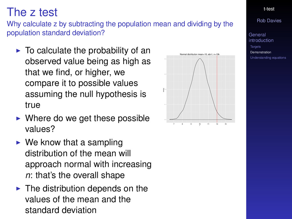
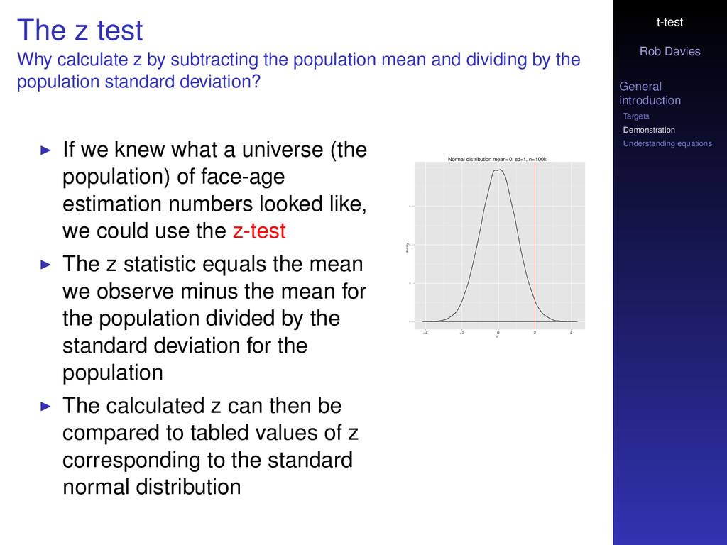
z test Why calculate z by subtracting the population mean and dividing by the population standard deviation? To calculate the probability of an observed value being as high as that we find, or higher, we compare it to possible values assuming the null hypothesis is true Where do we get these possible values? We know that a sampling distribution of the mean will approach normal with increasing n: that’s the overall shape The distribution depends on the values of the mean and the standard deviation Normal distribution mean=10, sd=1, n=10k z density 0.0 0.1 0.2 0.3 0.4 7 8 9 10 11 12 13
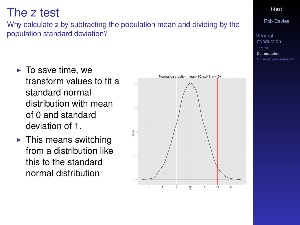
z test Why calculate z by subtracting the population mean and dividing by the population standard deviation? To save time, we transform values to fit a standard normal distribution with mean of 0 and standard deviation of 1. This means switching from a distribution like this to the standard normal distribution Normal distribution mean=10, sd=1, n=10k z density 0.0 0.1 0.2 0.3 0.4 7 8 9 10 11 12 13
z test Why calculate z by subtracting the population mean and dividing by the population standard deviation? If we knew what a universe (the population) of face-age estimation numbers looked like, we could use the z-test The z statistic equals the mean we observe minus the mean for the population divided by the standard deviation for the population The calculated z can then be compared to tabled values of z corresponding to the standard normal distribution Normal distribution mean=0, sd=1, n=100k z density 0.0 0.1 0.2 0.3 −4 −2 0 2 4
t test When we do not know—but have to assume—what the sampling distribution looks like We might always sample from a population but we rarely know the population µ or σ We need to compare the test statistic we calculate with values in the sampling distribution of t
t test When we do not know—but have to assume—what the sampling distribution looks like The t statistic equals the mean we observe minus the (hypothesized) mean for the population divided by the square root of the standard deviation of our sample, divided by n The calculated t statistic can then be compared to tabled values of t corresponding to the Student distribution of values of t . . . to calculate the probability of seeing a t as high as the one we calculated . . . assuming that the null hypothesis were true
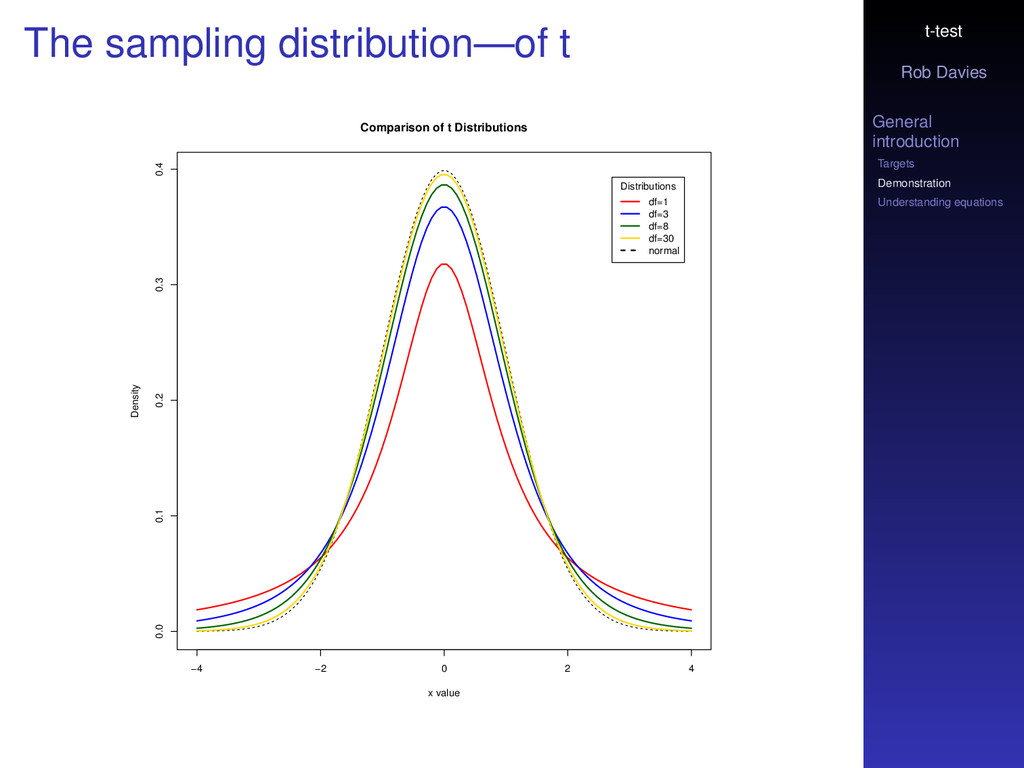
sampling distribution—of t We hardly ever know the mean and standard deviation of the population of numbers we are working with This is a problem especially in our ignorance about the standard deviation of the variation in the numbers We switch from working with the standard normal (z) distribution to working with the t distribution The problem arises because we do not know the population variance so have to use the sample variance s2 to characterize our distribution
sampling distribution—of t Treating the test statistic as a z score would not give a fair estimate of probability Because the s2 distribution is skewed so dividing a mean by it will give us a larger value than if we had used the true population variance William Gossett worked out in 1908 that if the data are sampled from a normal distribution using s2 would lead to a sampling distribution now called Student’s t distribution Because of Student’s work we can adapt the z distribution, use s2, calculate the answer now as t and compare it to the t distribution
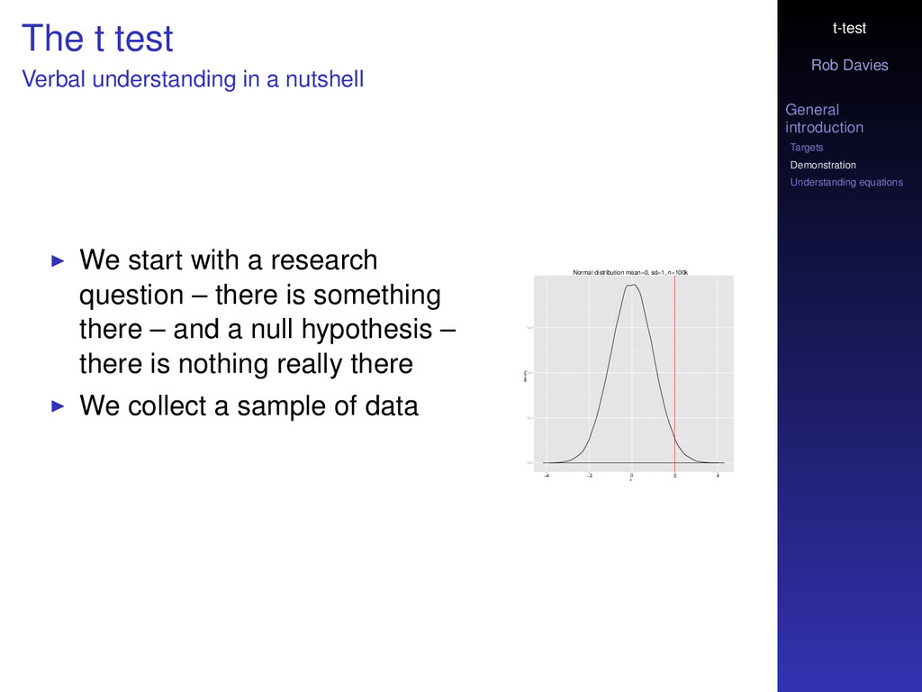
t test Verbal understanding in a nutshell We start with a research question – there is something there – and a null hypothesis – there is nothing really there We collect a sample of data Normal distribution mean=0, sd=1, n=100k z density 0.0 0.1 0.2 0.3 −4 −2 0 2 4
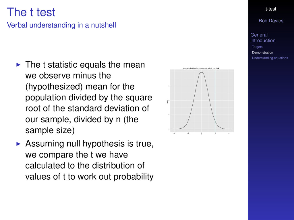
t test Verbal understanding in a nutshell The t statistic equals the mean we observe minus the (hypothesized) mean for the population divided by the square root of the standard deviation of our sample, divided by n (the sample size) Assuming null hypothesis is true, we compare the t we have calculated to the distribution of values of t to work out probability Normal distribution mean=0, sd=1, n=100k z density 0.0 0.1 0.2 0.3 −4 −2 0 2 4
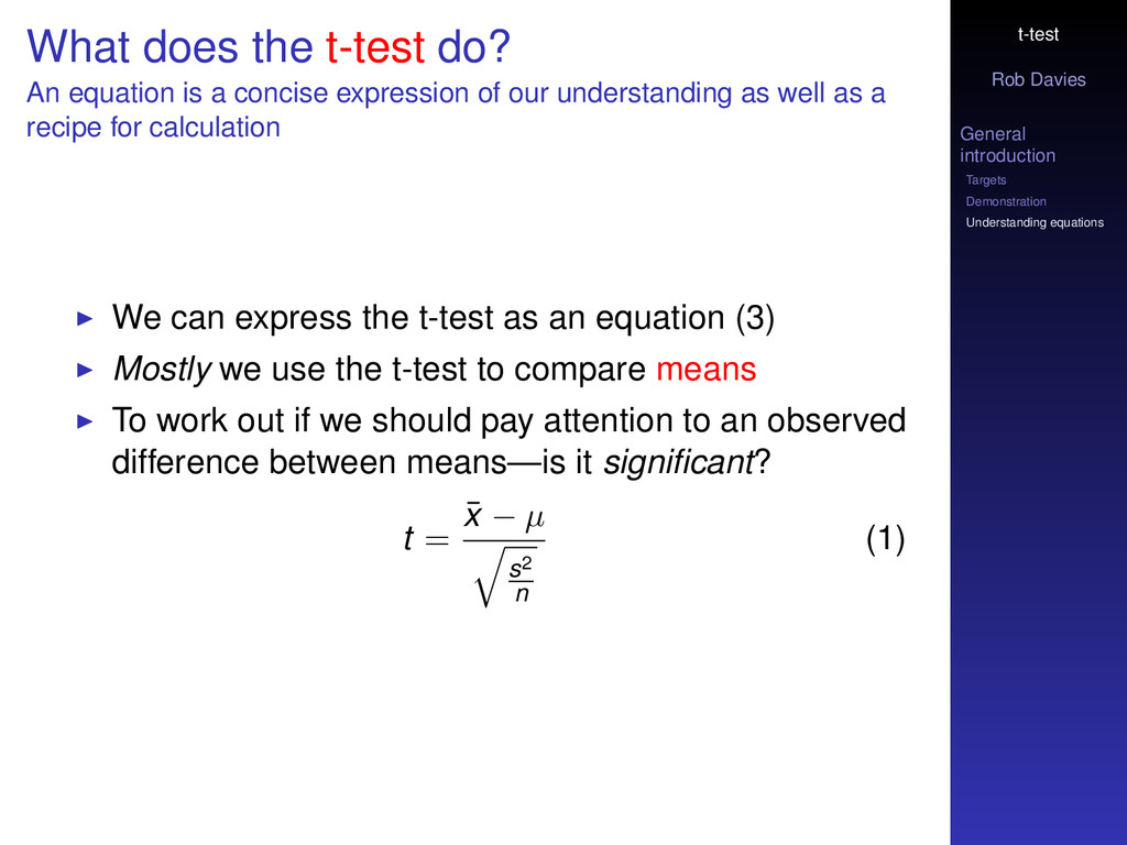
does the t-test do? An equation is a concise expression of our understanding as well as a recipe for calculation We can express the t-test as an equation (3) Mostly we use the t-test to compare means To work out if we should pay attention to an observed difference between means—is it significant? t = ¯ x − µ s2 n (1)
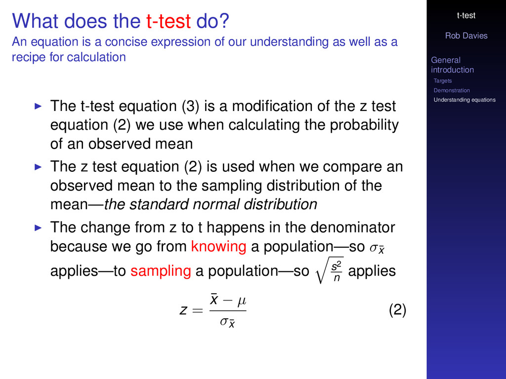
does the t-test do? An equation is a concise expression of our understanding as well as a recipe for calculation The t-test equation (3) is a modification of the z test equation (2) we use when calculating the probability of an observed mean The z test equation (2) is used when we compare an observed mean to the sampling distribution of the mean—the standard normal distribution The change from z to t happens in the denominator because we go from knowing a population—so σ¯ x applies—to sampling a population—so s2 n applies z = ¯ x − µ σ¯ x (2)
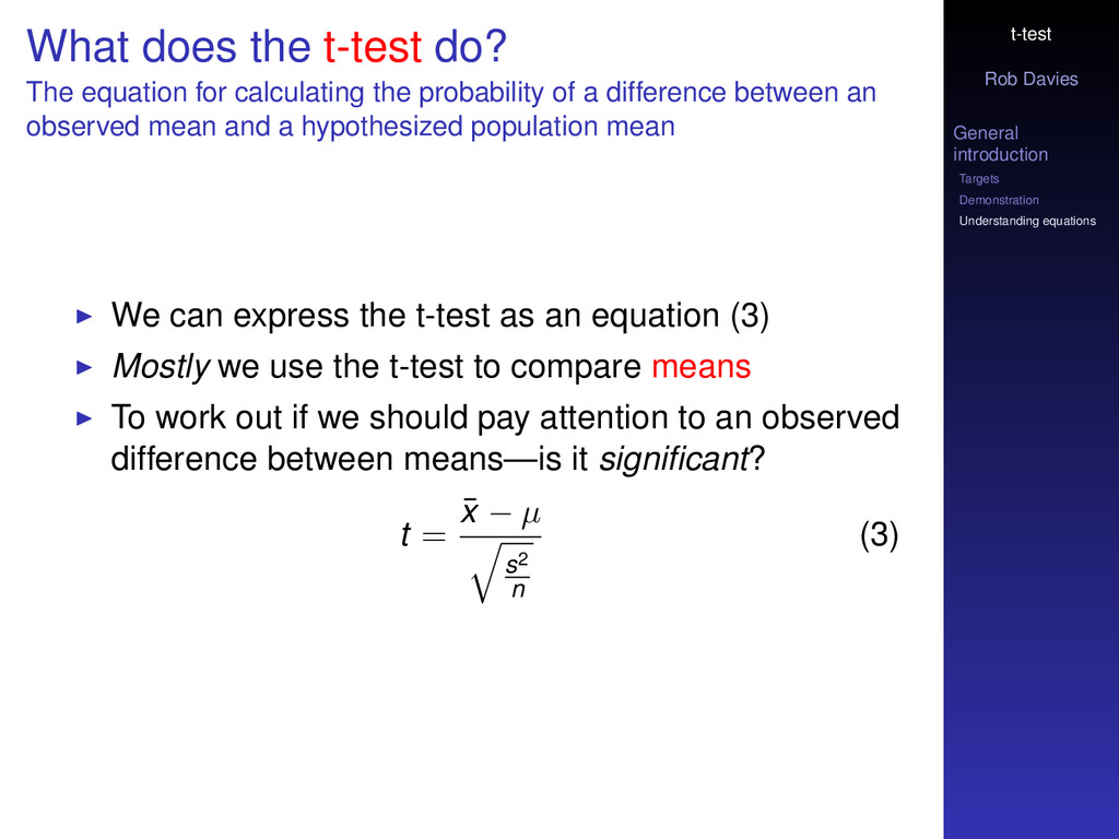
does the t-test do? The equation for calculating the probability of a difference between an observed mean and a hypothesized population mean We can express the t-test as an equation (3) Mostly we use the t-test to compare means To work out if we should pay attention to an observed difference between means—is it significant? t = ¯ x − µ s2 n (3)
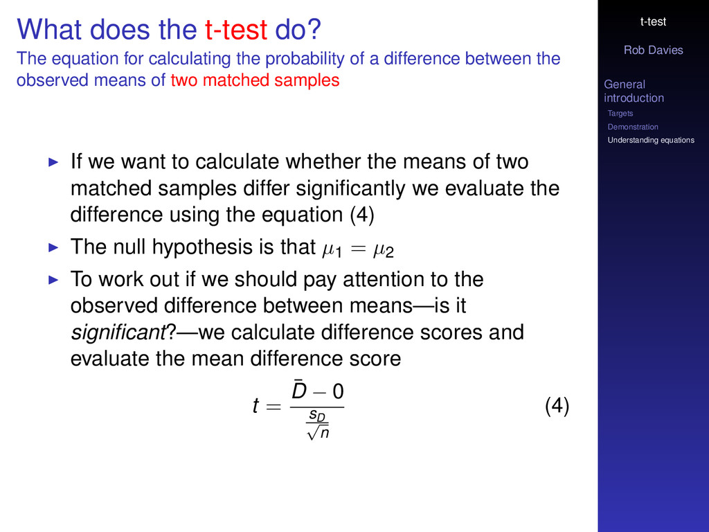
does the t-test do? The equation for calculating the probability of a difference between the observed means of two matched samples If we want to calculate whether the means of two matched samples differ significantly we evaluate the difference using the equation (4) The null hypothesis is that µ1 = µ2 To work out if we should pay attention to the observed difference between means—is it significant?—we calculate difference scores and evaluate the mean difference score t = ¯ D − 0 sD √ n (4)
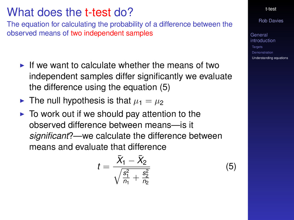
does the t-test do? The equation for calculating the probability of a difference between the observed means of two independent samples If we want to calculate whether the means of two independent samples differ significantly we evaluate the difference using the equation (5) The null hypothesis is that µ1 = µ2 To work out if we should pay attention to the observed difference between means—is it significant?—we calculate the difference between means and evaluate that difference t = ¯ X1 − ¯ X2 s2 1 n1 + s2 2 n2 (5)
key ideas you may have to deal with in analyses Key vocabulary Are samples matched or independent? What is the effect size? What are the confidence intervals?