Probing the final-parsec problem with pulsar-timing arrays

[07/07/2016] Seminar given at Radboud University, Netherlands.

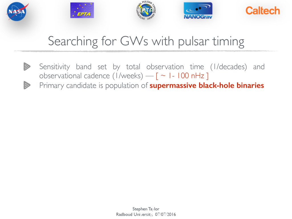
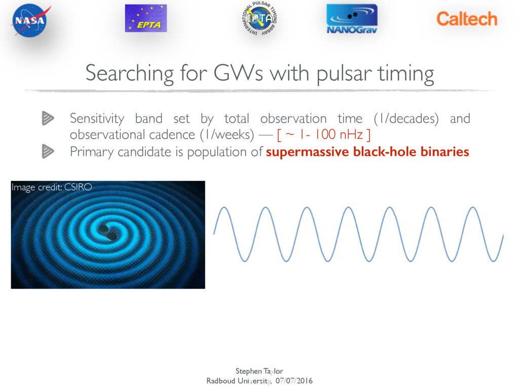
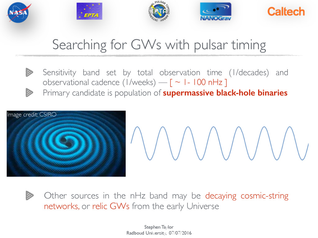
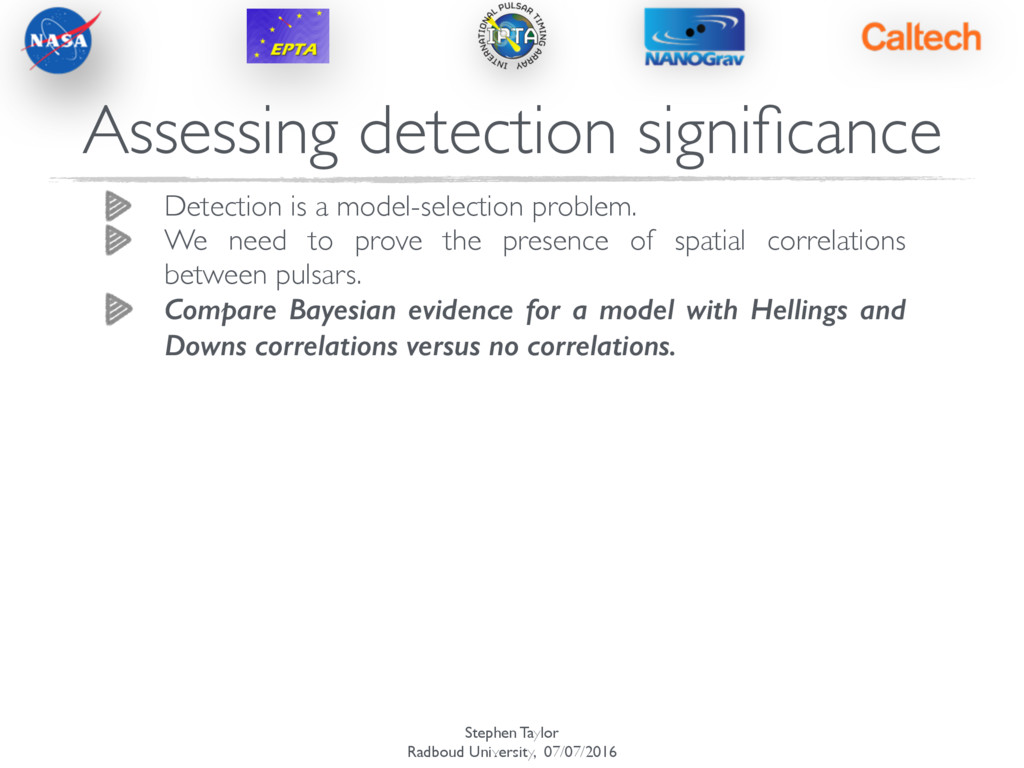
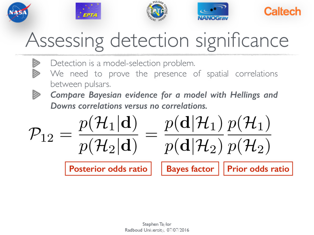
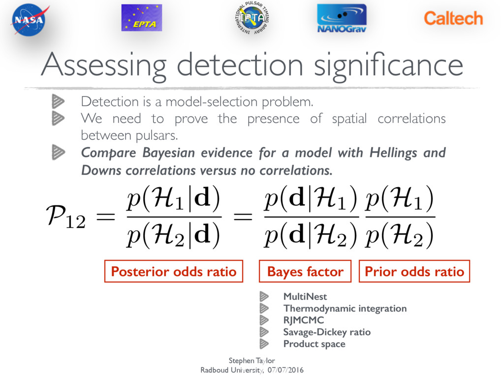
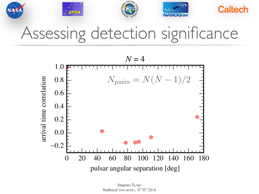
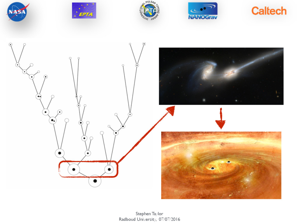
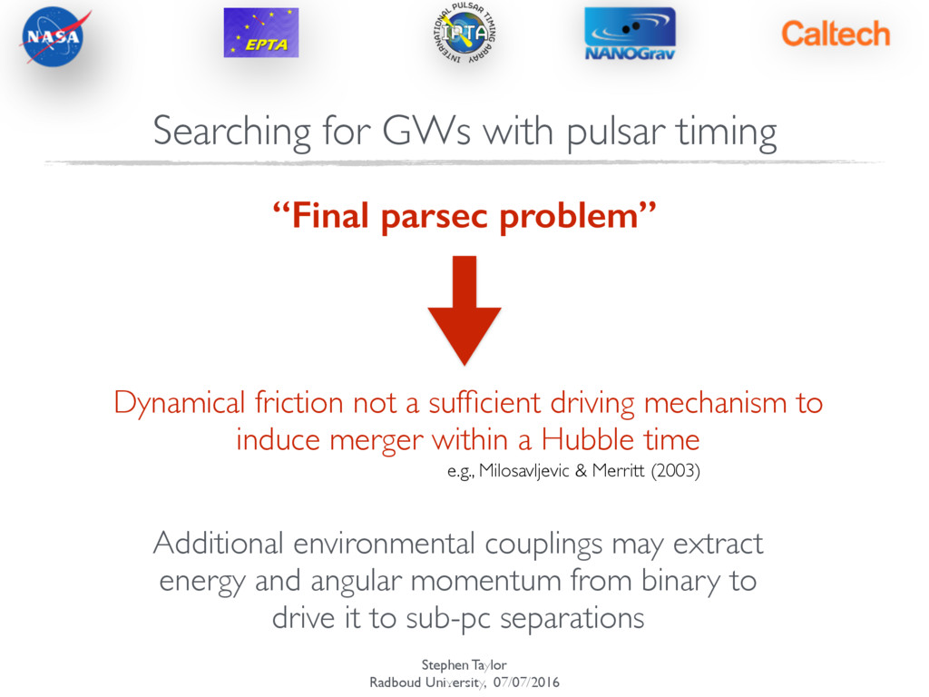
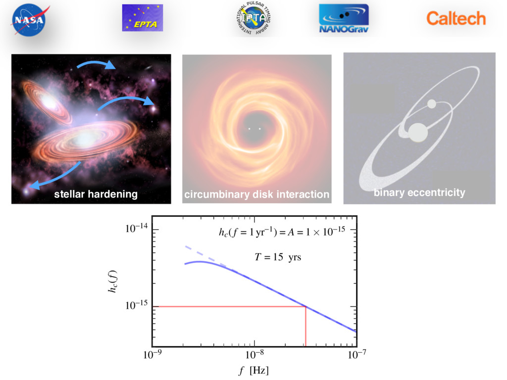
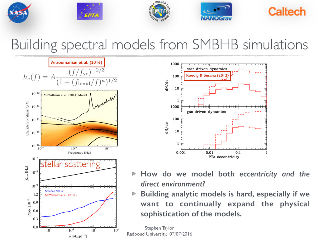
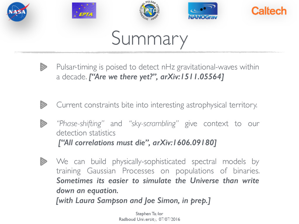
I give an overview of pulsar-timing searches for gravitational-waves, the expected source population, and how we can mine the shape of the gravitational-wave spectrum for details of the final-parsec of black-hole binary evolution.

Transcript

1. Stephen Taylor Radboud University, 07/07/2016 © 2016 California Institute of Technology. Government sponsorship acknowledged Stephen R. Taylor Probing the final-parsec problem with pulsar-timing arrays NASA POSTDOCTORAL FELLOW, JET PROPULSION LABORATORY, CALIFORNIA INSTITUTE OF TECHNOLOGY
2. Stephen Taylor Radboud University, 07/07/2016 Pulsars and pulsar-timing ! Searching for nanohertz GWs ! Assessing detection significance ! Final-parsec influences, and building search models from simulations Overview
3. Stephen Taylor Radboud University, 07/07/2016 Discovered in 1967 by Hewish, Bell, et al. ! Rapid rotation (P~1s), and strong magnetic field (~ G) ! Radio emission along magnetic field axis ! Misalignment of rotation and magnetic field axes creates lighthouse effect 1012 Image credit: Bill Saxton Pulsars
4. Stephen Taylor Radboud University, 07/07/2016 Discovered in 1967 by Hewish, Bell, et al. ! Rapid rotation (P~1s), and strong magnetic field (~ G) ! Radio emission along magnetic field axis ! Misalignment of rotation and magnetic field axes creates lighthouse effect 1012 Image credit: Bill Saxton Joeri van Leeuwen Pulsars
5. Stephen Taylor Radboud University, 07/07/2016 Pulsar timing ! Sophisticated timing models depend on P, Pdot, pulsar sky location, ISM properties, pulsar binary parameters etc….. Image credit: Duncan Lorimer
6. Stephen Taylor Radboud University, 07/07/2016 good timing-solution error in frequency derivative error in position unmodeled proper motion Lorimer & Kramer (2005)
7. Stephen Taylor Radboud University, 07/07/2016
8. Stephen Taylor Radboud University, 07/07/2016 John Rowe Animation/Australia Telescope National Facility, CSIRO
9. Stephen Taylor Radboud University, 07/07/2016
10. Stephen Taylor Radboud University, 07/07/2016 Sensitivity band set by total observation time (1/decades) and observational cadence (1/weeks) — [ ~ 1- 100 nHz ] Primary candidate is population of supermassive black-hole binaries Searching for GWs with pulsar timing
11. Stephen Taylor Radboud University, 07/07/2016 Sensitivity band set by total observation time (1/decades) and observational cadence (1/weeks) — [ ~ 1- 100 nHz ] Primary candidate is population of supermassive black-hole binaries Image credit: CSIRO Searching for GWs with pulsar timing
12. Stephen Taylor Radboud University, 07/07/2016 Sensitivity band set by total observation time (1/decades) and observational cadence (1/weeks) — [ ~ 1- 100 nHz ] Primary candidate is population of supermassive black-hole binaries Image credit: CSIRO Searching for GWs with pulsar timing
13. Stephen Taylor Radboud University, 07/07/2016 Sensitivity band set by total observation time (1/decades) and observational cadence (1/weeks) — [ ~ 1- 100 nHz ] Primary candidate is population of supermassive black-hole binaries Other sources in the nHz band may be decaying cosmic-string networks, or relic GWs from the early Universe Image credit: CSIRO Searching for GWs with pulsar timing
14. Stephen Taylor Radboud University, 07/07/2016 Image credit: David Champion
15. Stephen Taylor Radboud University, 07/07/2016 Image credit: David Champion Hellings & Downs (1983)
16. Stephen Taylor Radboud University, 07/07/2016 Assessing detection significance Detection is a model-selection problem. We need to prove the presence of spatial correlations between pulsars. Compare Bayesian evidence for a model with Hellings and Downs correlations versus no correlations.
17. Stephen Taylor Radboud University, 07/07/2016 Assessing detection significance Detection is a model-selection problem. We need to prove the presence of spatial correlations between pulsars. Compare Bayesian evidence for a model with Hellings and Downs correlations versus no correlations. P12 = p(H1 |d) p(H2 |d) = p(d|H1) p(d|H2) p(H1) p(H2) Posterior odds ratio Bayes factor Prior odds ratio
18. Stephen Taylor Radboud University, 07/07/2016 Assessing detection significance Detection is a model-selection problem. We need to prove the presence of spatial correlations between pulsars. Compare Bayesian evidence for a model with Hellings and Downs correlations versus no correlations. P12 = p(H1 |d) p(H2 |d) = p(d|H1) p(d|H2) p(H1) p(H2) Posterior odds ratio Bayes factor Prior odds ratio MultiNest Thermodynamic integration RJMCMC Savage-Dickey ratio Product space
19. Stephen Taylor Radboud University, 07/07/2016 0 20 40 60 80 100 120 140 160 180 pulsar angular separation [deg] -0.2 0.0 0.2 0.4 0.6 0.8 1.0 arrival time correlation N = 1 Npairs = N(N 1)/2 Assessing detection significance
20. Stephen Taylor Radboud University, 07/07/2016 0 20 40 60 80 100 120 140 160 180 pulsar angular separation [deg] -0.2 0.0 0.2 0.4 0.6 0.8 1.0 arrival time correlation N = 1 0 20 40 60 80 100 120 140 160 180 pulsar angular separation [deg] -0.2 0.0 0.2 0.4 0.6 0.8 1.0 arrival time correlation N = 4 Npairs = N(N 1)/2 Assessing detection significance
21. Stephen Taylor Radboud University, 07/07/2016 0 20 40 60 80 100 120 140 160 180 pulsar angular separation [deg] -0.2 0.0 0.2 0.4 0.6 0.8 1.0 arrival time correlation N = 1 0 20 40 60 80 100 120 140 160 180 pulsar angular separation [deg] -0.2 0.0 0.2 0.4 0.6 0.8 1.0 arrival time correlation N = 4 0 20 40 60 80 100 120 140 160 180 pulsar angular separation [deg] -0.2 0.0 0.2 0.4 0.6 0.8 1.0 arrival time correlation N = 10 Npairs = N(N 1)/2 Assessing detection significance
22. Stephen Taylor Radboud University, 07/07/2016 0 20 40 60 80 100 120 140 160 180 pulsar angular separation [deg] -0.2 0.0 0.2 0.4 0.6 0.8 1.0 arrival time correlation N = 1 0 20 40 60 80 100 120 140 160 180 pulsar angular separation [deg] -0.2 0.0 0.2 0.4 0.6 0.8 1.0 arrival time correlation N = 4 0 20 40 60 80 100 120 140 160 180 pulsar angular separation [deg] -0.2 0.0 0.2 0.4 0.6 0.8 1.0 arrival time correlation N = 10 0 20 40 60 80 100 120 140 160 180 pulsar angular separation [deg] -0.2 0.0 0.2 0.4 0.6 0.8 1.0 arrival time correlation N = 30 Npairs = N(N 1)/2 Assessing detection significance
23. Stephen Taylor Radboud University, 07/07/2016 0 20 40 60 80 100 120 140 160 180 pulsar angular separation [deg] -0.2 0.0 0.2 0.4 0.6 0.8 1.0 arrival time correlation N = 1 0 20 40 60 80 100 120 140 160 180 pulsar angular separation [deg] -0.2 0.0 0.2 0.4 0.6 0.8 1.0 arrival time correlation N = 4 0 20 40 60 80 100 120 140 160 180 pulsar angular separation [deg] -0.2 0.0 0.2 0.4 0.6 0.8 1.0 arrival time correlation N = 10 0 20 40 60 80 100 120 140 160 180 pulsar angular separation [deg] -0.2 0.0 0.2 0.4 0.6 0.8 1.0 arrival time correlation N = 30 0 20 40 60 80 100 120 140 160 180 pulsar angular separation [deg] -0.2 0.0 0.2 0.4 0.6 0.8 1.0 arrival time correlation N = 50 Npairs = N(N 1)/2 Assessing detection significance
24. Stephen Taylor Radboud University, 07/07/2016 0 5 10 PPTA4 0 20 40 60 80 100 NANOGrav+ 0 20 40 60 80 100 EPTA+ 0 20 40 60 80 100 IPTA+ 0 5 10 15 20 T [yrs] 0 20 40 60 80 100 TPTA Expected detection probability [%] Taylor et al. (2016a), ApJL 819, L6
25. Stephen Taylor Radboud University, 07/07/2016 Detection statistic (whether frequentist or Bayesian) needs context. How often can noise alone produce this? Could run many noise simulations to determine p-value of measured statistic… Better to operate on real dataset. Assessing detection significance
26. Stephen Taylor Radboud University, 07/07/2016 Cgwb = F'gwbFT Phase Shifting Sky Scrambles …also see Cornish & Sampson (2016) for discussions of how to make robust detections Detection statistic (whether frequentist or Bayesian) needs context. How often can noise alone produce this? Could run many noise simulations to determine p-value of measured statistic… Better to operate on real dataset. “All correlations must die” , Taylor et al. (2016b), arXiv:1606.09180 Assessing detection significance
27. Stephen Taylor Radboud University, 07/07/2016 -60 -50 -40 -30 -20 -10 0 lnB 0.00 0.02 0.04 0.06 0.08 0.10 Common uncorrelated red process GWB signal, scrambled ORF GWB signal, phase shifts Phase-shifting: add random phases to all basis functions of GWB signal. ! Sky-scrambling: scramble pulsar positions when constructing the Hellings & Downs curve in our model, to be orthogonal to the true Hellings & Downs curve. Assessing detection significance
28. Stephen Taylor Radboud University, 07/07/2016
29. Stephen Taylor Radboud University, 07/07/2016
30. Stephen Taylor Radboud University, 07/07/2016
31. Stephen Taylor Radboud University, 07/07/2016 “Final parsec problem” Dynamical friction not a sufficient driving mechanism to induce merger within a Hubble time e.g., Milosavljevic & Merritt (2003) Searching for GWs with pulsar timing
32. Stephen Taylor Radboud University, 07/07/2016 “Final parsec problem” Dynamical friction not a sufficient driving mechanism to induce merger within a Hubble time e.g., Milosavljevic & Merritt (2003) Additional environmental couplings may extract energy and angular momentum from binary to drive it to sub-pc separations Searching for GWs with pulsar timing
33. Stephen Taylor Radboud University, 07/07/2016
34. Stephen Taylor Radboud University, 07/07/2016 circumbinary disk interaction stellar hardening binary eccentricity
35. Stephen Taylor Radboud University, 07/07/2016 circumbinary disk interaction stellar hardening binary eccentricity 10-9 10-8 10-7 f [Hz] 10-15 10-14 hc(f) hc(f = 1yr-1) = A = 1⇥10-15 T = 9 yrs
36. Stephen Taylor Radboud University, 07/07/2016 circumbinary disk interaction stellar hardening binary eccentricity 10-9 10-8 10-7 f [Hz] 10-15 10-14 hc(f) hc(f = 1yr-1) = A = 1⇥10-15 T = 9 yrs 10-9 10-8 10-7 f [Hz] 10-15 10-14 hc(f) hc(f = 1yr-1) = A = 1⇥10-15 T = 11 yrs
37. Stephen Taylor Radboud University, 07/07/2016 circumbinary disk interaction stellar hardening binary eccentricity 10-9 10-8 10-7 f [Hz] 10-15 10-14 hc(f) hc(f = 1yr-1) = A = 1⇥10-15 T = 9 yrs 10-9 10-8 10-7 f [Hz] 10-15 10-14 hc(f) hc(f = 1yr-1) = A = 1⇥10-15 T = 11 yrs 10-9 10-8 10-7 f [Hz] 10-15 10-14 hc(f) hc(f = 1yr-1) = A = 1⇥10-15 T = 15 yrs
38. Stephen Taylor Radboud University, 07/07/2016 circumbinary disk interaction stellar hardening binary eccentricity 10-9 10-8 10-7 f [Hz] 10-15 10-14 hc(f) hc(f = 1yr-1) = A = 1⇥10-15 T = 9 yrs 10-9 10-8 10-7 f [Hz] 10-15 10-14 hc(f) hc(f = 1yr-1) = A = 1⇥10-15 T = 11 yrs 10-9 10-8 10-7 f [Hz] 10-15 10-14 hc(f) hc(f = 1yr-1) = A = 1⇥10-15 T = 15 yrs 10-9 10-8 10-7 f [Hz] 10-15 10-14 hc(f) hc(f = 1yr-1) = A = 1⇥10-15 T = 30 yrs
39. Stephen Taylor Radboud University, 07/07/2016 Building spectral models from SMBHB simulations 12 10-9 10-8 10-7 Frequency [Hz] 10-16 10-15 10-14 10-13 10-12 Characteristic Strain [hc(f)] McWilliams et al. (2014) Model Figure 5. Probability density plots of the recovered GWB spectra for models A and B using the broken-power-law model parameterized by (Agw, fbend, and ) as discussed in the text. The thick black lines indicate the 95% credible region and median of the GWB spectrum. The dashed line shows the 95% upper limit on the amplitude of purely GW-driven spectrum using the Gaussian priors on the amplitude from models A and B, respectively. The thin black curve shows the 95% upper limit on the GWB spectrum from the spectral analysis. 16 10-9 10-8 10-7 fturn [Hz] 103 104 105 106 ⇢ [M pc-3] 0.0 0.3 0.6 0.9 1.2 Prob. [10-6] Sesana (2013) McWilliams et al. (2014) stellar scattering hc(f) = A (f/fyr) 2/3 (1 + (fbend/f))1/2 Arzoumanian et al. (2016)
40. Stephen Taylor Radboud University, 07/07/2016 Building spectral models from SMBHB simulations 12 10-9 10-8 10-7 Frequency [Hz] 10-16 10-15 10-14 10-13 10-12 Characteristic Strain [hc(f)] McWilliams et al. (2014) Model Figure 5. Probability density plots of the recovered GWB spectra for models A and B using the broken-power-law model parameterized by (Agw, fbend, and ) as discussed in the text. The thick black lines indicate the 95% credible region and median of the GWB spectrum. The dashed line shows the 95% upper limit on the amplitude of purely GW-driven spectrum using the Gaussian priors on the amplitude from models A and B, respectively. The thin black curve shows the 95% upper limit on the GWB spectrum from the spectral analysis. 16 10-9 10-8 10-7 fturn [Hz] 103 104 105 106 ⇢ [M pc-3] 0.0 0.3 0.6 0.9 1.2 Prob. [10-6] Sesana (2013) McWilliams et al. (2014) stellar scattering hc(f) = A (f/fyr) 2/3 (1 + (fbend/f))1/2 Figure 2. Eccentricity population of MBHBs detectable by ELISA/NGO and PTAs, expected in stellar and gaseous environments. Left panel: The solid histograms represent the efficient models whereas the dashed histograms are for the inefficient models. Right panel: solid his- tograms include all sources producing timing residuals above 3 ns, dashed histograms include all sources producing residual above 10 ns. mechanism (gas/star) we consider two scenarios (efficient/inefficient), to give an idea of the expected eccentricity range. The models are the following (i) gas-efficient: α = 0.3, ˙ m = 1. The migration timescale is maximized for this high values of the disc parameters, and the decoupling occurs in the very late stage of the MBHB evolution; Roedig & Sesana (2012) Arzoumanian et al. (2016)
41. Stephen Taylor Radboud University, 07/07/2016 Building spectral models from SMBHB simulations 12 10-9 10-8 10-7 Frequency [Hz] 10-16 10-15 10-14 10-13 10-12 Characteristic Strain [hc(f)] McWilliams et al. (2014) Model Figure 5. Probability density plots of the recovered GWB spectra for models A and B using the broken-power-law model parameterized by (Agw, fbend, and ) as discussed in the text. The thick black lines indicate the 95% credible region and median of the GWB spectrum. The dashed line shows the 95% upper limit on the amplitude of purely GW-driven spectrum using the Gaussian priors on the amplitude from models A and B, respectively. The thin black curve shows the 95% upper limit on the GWB spectrum from the spectral analysis. 16 10-9 10-8 10-7 fturn [Hz] 103 104 105 106 ⇢ [M pc-3] 0.0 0.3 0.6 0.9 1.2 Prob. [10-6] Sesana (2013) McWilliams et al. (2014) stellar scattering hc(f) = A (f/fyr) 2/3 (1 + (fbend/f))1/2 Figure 2. Eccentricity population of MBHBs detectable by ELISA/NGO and PTAs, expected in stellar and gaseous environments. Left panel: The solid histograms represent the efficient models whereas the dashed histograms are for the inefficient models. Right panel: solid his- tograms include all sources producing timing residuals above 3 ns, dashed histograms include all sources producing residual above 10 ns. mechanism (gas/star) we consider two scenarios (efficient/inefficient), to give an idea of the expected eccentricity range. The models are the following (i) gas-efficient: α = 0.3, ˙ m = 1. The migration timescale is maximized for this high values of the disc parameters, and the decoupling occurs in the very late stage of the MBHB evolution; Roedig & Sesana (2012) Arzoumanian et al. (2016) How do we model both eccentricity and the direct environment? Building analytic models is hard, especially if we want to continually expand the physical sophistication of the models.
42. Stephen Taylor Radboud University, 07/07/2016 Building spectral models from SMBHB simulations
43. Stephen Taylor Radboud University, 07/07/2016 Gaussian Process Interpolation •Run a small number of expensive SMBHB population simulations. •Learn the shape of the spectrum at different physical parameter values. •Learn the spectral variance due to finiteness of the SMBHB population. ! •We have a predictor for the shape of the spectrum, AND a measure of the uncertainty from the interpolation scheme. Building spectral models from SMBHB simulations
44. Stephen Taylor Radboud University, 07/07/2016 10-8 10-7 f [Hz] 10-1 100 101 hc(f) ⇢ = 100M pc-3 ⇢ = 500 ⇢ = 1000 ⇢ = 105 ⇢ = 106 /Ah /Ah Building spectral models from SMBHB simulations
45. Stephen Taylor Radboud University, 07/07/2016 10-8 10-7 f [Hz] 10-1 100 101 hc(f) ⇢ = 100M pc-3 ⇢ = 500 ⇢ = 1000 ⇢ = 105 ⇢ = 106 /Ah 10-8 10-7 f [Hz] 10-1 100 101 hc(f) ⇢ = 100M pc-3 ⇢ = 500 ⇢ = 1000 ⇢ = 105 ⇢ = 106 /Ah Building spectral models from SMBHB simulations
46. Stephen Taylor Radboud University, 07/07/2016 • Gaussian Process trained at a few stellar density values. • We can predict the spectral shape at any stellar density value! • Carry the interpolation uncertainty forward into our GW inference. 6 8 10 12 1 1 2 3 4 5 2 1 2 3 4 5 2 x = log10 ⇢ y = log10( Sh( f ) /A2 h) ln LGP = 1 2 ln det(2⇡K) 1 2 yT K 1y Kij = K ( xi, xj) Building spectral models from SMBHB simulations
47. Stephen Taylor Radboud University, 07/07/2016 • Gaussian Process trained at a few stellar density values. • We can predict the spectral shape at any stellar density value! • Carry the interpolation uncertainty forward into our GW inference. 6 8 10 12 1 1 2 3 4 5 2 1 2 3 4 5 2 0 1 2 3 4 5 6 log10 ⇢ 0.000 0.002 0.004 0.006 0.008 0.010 0.012 0.014 0.016 % uncertainty f =35.04 nHz x = log10 ⇢ y = log10( Sh( f ) /A2 h) ln LGP = 1 2 ln det(2⇡K) 1 2 yT K 1y Kij = K ( xi, xj) Building spectral models from SMBHB simulations
48. Stephen Taylor Radboud University, 07/07/2016 -14.4 -14.0 -13.6 log10 Agwb 1.5 3.0 4.5 6.0 log10 ⇢ 1.5 3.0 4.5 6.0 log10 ⇢ Green = analysis with exactly- known spectral model Red = analysis with GP model
49. Stephen Taylor Radboud University, 07/07/2016 10-8 10-7 f [Hz] 10-17 10-16 10-15 10-14 hc(f) e0 = 0 e0 = 0.2 e0 = 0.3 e0 = 0.4 e0 = 0.5 e0 = 0.6 e0 = 0.7 e0 = 0.8 e0 = 0.9
50. Stephen Taylor Radboud University, 07/07/2016 10-8 10-7 f [Hz] 10-17 10-16 10-15 10-14 hc(f) e0 = 0 e0 = 0.2 e0 = 0.3 e0 = 0.4 e0 = 0.5 e0 = 0.6 e0 = 0.7 e0 = 0.8 e0 = 0.9 log10 Agwb = -13.32+0.11 -0.12 -13.6 -13.4 -13.2 -13.0 log10 Agwb 0.68 0.72 0.76 0.80 0.84 e0 0.68 0.72 0.76 0.80 0.84 e0 e0 = 0.77+0.02 -0.03
51. Stephen Taylor Radboud University, 07/07/2016 Summary Pulsar-timing is poised to detect nHz gravitational-waves within a decade. [“Are we there yet?”, arXiv:1511.05564] ! ! Current constraints bite into interesting astrophysical territory. ! “Phase-shifting” and “sky-scrambling” give context to our detection statistics [“All correlations must die”, arXiv:1606.09180] ! We can build physically-sophisticated spectral models by training Gaussian Processes on populations of binaries. Sometimes its easier to simulate the Universe than write down an equation. [with Laura Sampson and Joe Simon, in prep.]