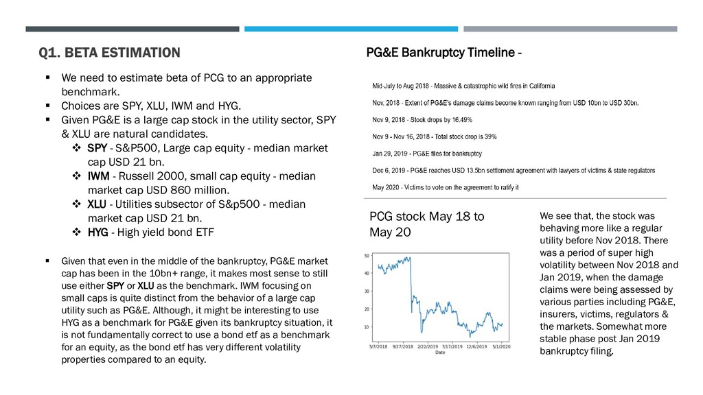
PCG to an appropriate benchmark. ▪ Choices are SPY, XLU, IWM and HYG. ▪ Given PG&E is a large cap stock in the utility sector, SPY & XLU are natural candidates. ❖ SPY - S&P500, Large cap equity - median market cap USD 21 bn. ❖ IWM - Russell 2000, small cap equity - median market cap USD 860 million. ❖ XLU - Utilities subsector of S&p500 - median market cap USD 21 bn. ❖ HYG - High yield bond ETF ▪ Given that even in the middle of the bankruptcy, PG&E market cap has been in the 10bn+ range, it makes most sense to still use either SPY or XLU as the benchmark. IWM focusing on small caps is quite distinct from the behavior of a large cap utility such as PG&E. Although, it might be interesting to use HYG as a benchmark for PG&E given its bankruptcy situation, it is not fundamentally correct to use a bond etf as a benchmark for an equity, as the bond etf has very different volatility properties compared to an equity. PG&E Bankruptcy Timeline - PCG stock May 18 to May 20 We see that, the stock was behaving more like a regular utility before Nov 2018. There was a period of super high volatility between Nov 2018 and Jan 2019, when the damage claims were being assessed by various parties including PG&E, insurers, victims, regulators & the markets. Somewhat more stable phase post Jan 2019 bankruptcy filing.
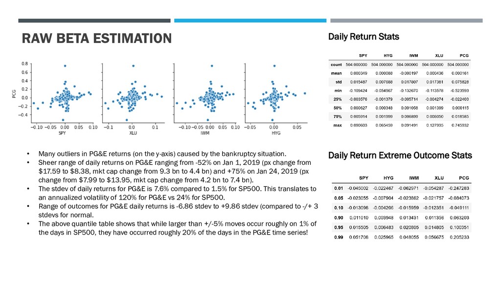
the y-axis) caused by the bankruptcy situation. • Sheer range of daily returns on PG&E ranging from -52% on Jan 1, 2019 (px change from $17.59 to $8.38, mkt cap change from 9.3 bn to 4.4 bn) and +75% on Jan 24, 2019 (px change from $7.99 to $13.95, mkt cap change from 4.2 bn to 7.4 bn). • The stdev of daily returns for PG&E is 7.6% compared to 1.5% for SP500. This translates to an annualized volatility of 120% for PG&E vs 24% for SP500. • Range of outcomes for PG&E daily returns is -6.86 stdev to +9.86 stdev (compared to -/+ 3 stdevs for normal. • The above quantile table shows that while larger than +/-5% moves occur roughly on 1% of the days in SP500, they have occurred roughly 20% of the days in the PG&E time series! Daily Return Stats Daily Return Extreme Outcome Stats
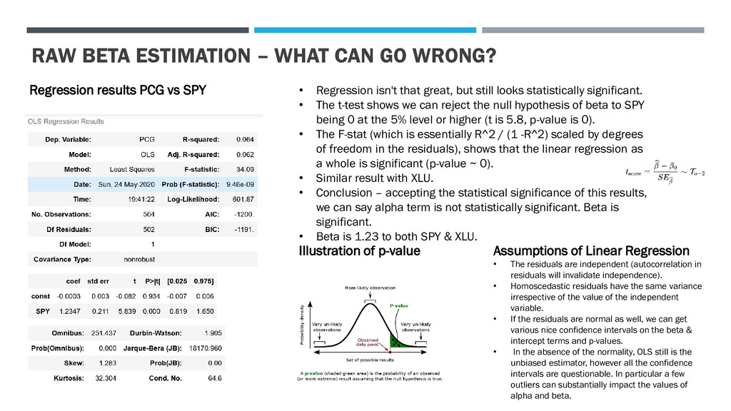
PCG vs SPY • Regression isn't that great, but still looks statistically significant. • The t-test shows we can reject the null hypothesis of beta to SPY being 0 at the 5% level or higher (t is 5.8, p-value is 0). • The F-stat (which is essentially R^2 / (1 -R^2) scaled by degrees of freedom in the residuals), shows that the linear regression as a whole is significant (p-value ~ 0). • Similar result with XLU. • Conclusion – accepting the statistical significance of this results, we can say alpha term is not statistically significant. Beta is significant. • Beta is 1.23 to both SPY & XLU. Illustration of p-value Assumptions of Linear Regression • The residuals are independent (autocorrelation in residuals will invalidate independence). • Homoscedastic residuals have the same variance irrespective of the value of the independent variable. • If the residuals are normal as well, we can get various nice confidence intervals on the beta & intercept terms and p-values. • In the absence of the normality, OLS still is the unbiased estimator, however all the confidence intervals are questionable. In particular a few outliers can substantially impact the values of alpha and beta.
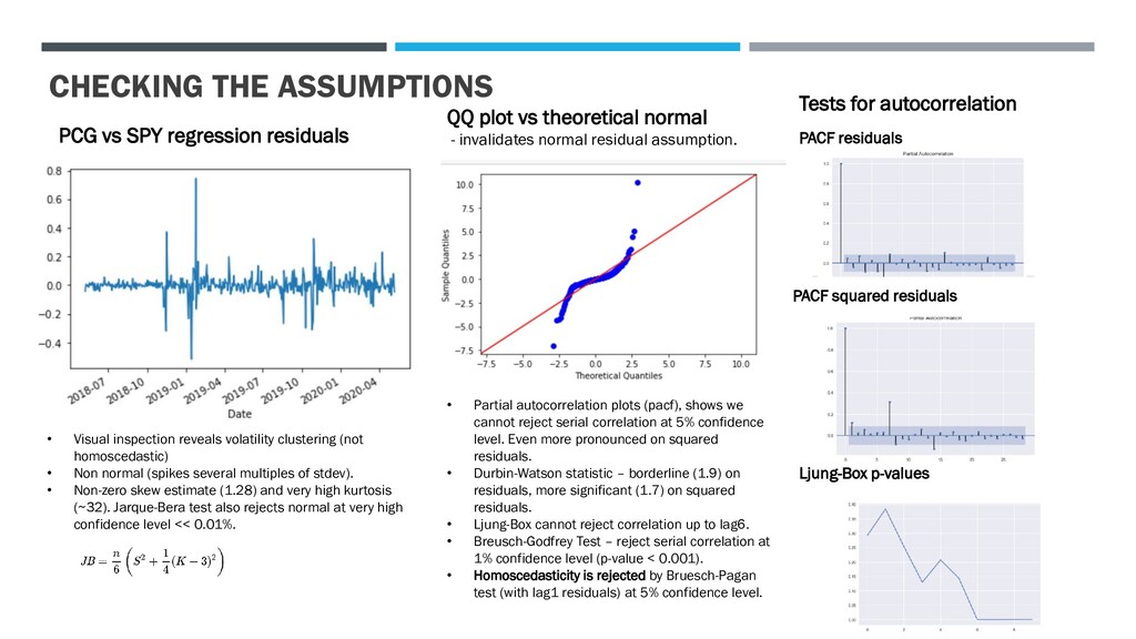
inspection reveals volatility clustering (not homoscedastic) • Non normal (spikes several multiples of stdev). • Non-zero skew estimate (1.28) and very high kurtosis (~32). Jarque-Bera test also rejects normal at very high confidence level << 0.01%. QQ plot vs theoretical normal - invalidates normal residual assumption. Tests for autocorrelation • Partial autocorrelation plots (pacf), shows we cannot reject serial correlation at 5% confidence level. Even more pronounced on squared residuals. • Durbin-Watson statistic – borderline (1.9) on residuals, more significant (1.7) on squared residuals. • Ljung-Box cannot reject correlation up to lag6. • Breusch-Godfrey Test – reject serial correlation at 1% confidence level (p-value < 0.001). • Homoscedasticity is rejected by Bruesch-Pagan test (with lag1 residuals) at 5% confidence level. PACF residuals PACF squared residuals Ljung-Box p-values
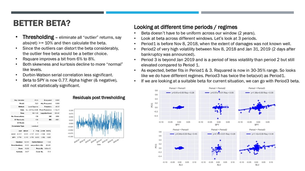
abs(ret) >= 10% and then calculate the beta. • Since the outliers can distort the beta considerably, the outlier free beta would be a better choice. • Rsquare improves a bit from 6% to 8%. • Both skewness and kurtosis decline to more “normal” like levels. • Durbin-Watson serial correlation less significant. • Beta to SPY is now 0.77. Alpha higher (& negative), still not statistically significant. Looking at different time periods / regimes • Beta doesn’t have to be uniform across our window (2 years). • Look at beta across different windows. Let’s look at 3 periods. • Period1 is before Nov 8, 2018, when the extent of damages was not known well. • Period2 of very high volatility between Nov 8, 2018 and Jan 31, 2019 (2 days after bankruptcy was announced). • Period 3 is beyond Jan 2019 and is a period of less volatility than period 2 but still elevated compared to Period 1. • As expected, better fits in Period1 & 3. Rsquared is now in 30-35% range. So looks like we do have different regimes. Period3 has twice the beta(vol) as Period1. • If we are looking at a suitable beta for current situation, we can go with Period3 beta. Residuals post thresholding
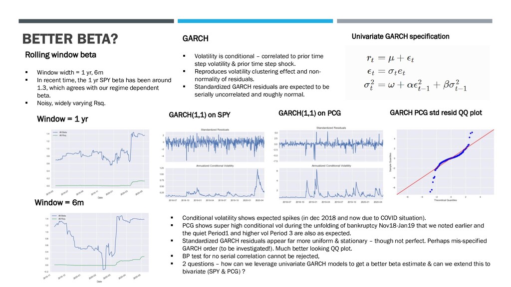
yr, 6m ▪ In recent time, the 1 yr SPY beta has been around 1.3, which agrees with our regime dependent beta. ▪ Noisy, widely varying Rsq. Window = 1 yr Window = 6m GARCH ▪ Volatility is conditional – correlated to prior time step volatility & prior time step shock. ▪ Reproduces volatility clustering effect and non- normality of residuals. ▪ Standardized GARCH residuals are expected to be serially uncorrelated and roughly normal. GARCH(1,1) on SPY GARCH(1,1) on PCG Univariate GARCH specification ▪ Conditional volatility shows expected spikes (in dec 2018 and now due to COVID situation). ▪ PCG shows super high conditional vol during the unfolding of bankruptcy Nov18-Jan19 that we noted earlier and the quiet Period1 and higher vol Period 3 are also as expected. ▪ Standardized GARCH residuals appear far more uniform & stationary – though not perfect. Perhaps mis-specified GARCH order (to be investigated!). Much better looking QQ plot. ▪ BP test for no serial correlation cannot be rejected, ▪ 2 questions – how can we leverage univariate GARCH models to get a better beta estimate & can we extend this to bivariate (SPY & PCG) ? GARCH PCG std resid QQ plot
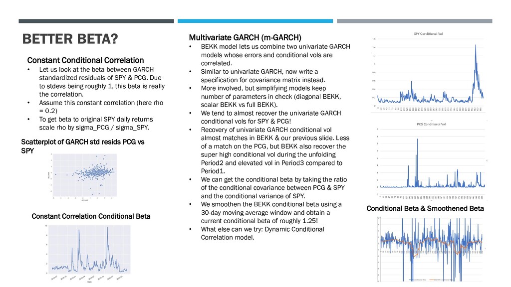
the beta between GARCH standardized residuals of SPY & PCG. Due to stdevs being roughly 1, this beta is really the correlation. • Assume this constant correlation (here rho = 0.2) • To get beta to original SPY daily returns scale rho by sigma_PCG / sigma_SPY. Constant Correlation Conditional Beta Scatterplot of GARCH std resids PCG vs SPY Multivariate GARCH (m-GARCH) • BEKK model lets us combine two univariate GARCH models whose errors and conditional vols are correlated. • Similar to univariate GARCH, now write a specification for covariance matrix instead. • More involved, but simplifying models keep number of parameters in check (diagonal BEKK, scalar BEKK vs full BEKK). • We tend to almost recover the univariate GARCH conditional vols for SPY & PCG! • Recovery of univariate GARCH conditional vol almost matches in BEKK & our previous slide. Less of a match on the PCG, but BEKK also recover the super high conditional vol during the unfolding Period2 and elevated vol in Period3 compared to Period1. • We can get the conditional beta by taking the ratio of the conditional covariance between PCG & SPY and the conditional variance of SPY. • We smoothen the BEKK conditional beta using a 30-day moving average window and obtain a current conditional beta of roughly 1.25! • What else can we try: Dynamic Conditional Correlation model. Conditional Beta & Smoothened Beta
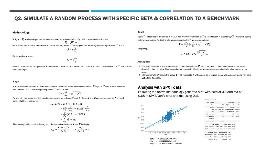
TO A BENCHMARK Analysis with SPXT data Following the above methodology generate a Y1 with beta of 0.3 and rho of 0.65 to SPXT. Verify beta and rho using OLS.
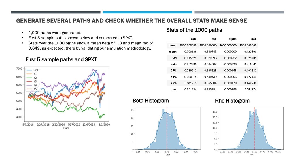
SENSE • 1,000 paths were generated. • First 5 sample paths shown below and compared to SPXT. • Stats over the 1000 paths show a mean beta of 0.3 and mean rho of 0.649, as expected, there by validating our simulation methodology. Stats of the 1000 paths First 5 sample paths and SPXT Beta Histogram Rho Histogram
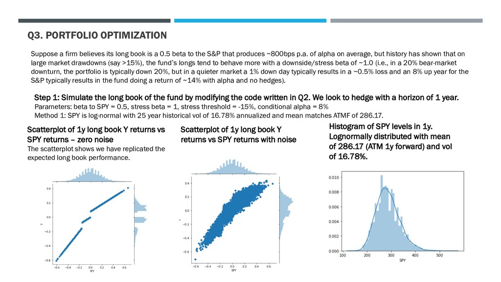
is a 0.5 beta to the S&P that produces ~800bps p.a. of alpha on average, but history has shown that on large market drawdowns (say >15%), the fund’s longs tend to behave more with a downside/stress beta of ~1.0 (i.e., in a 20% bear-market downturn, the portfolio is typically down 20%, but in a quieter market a 1% down day typically results in a ~0.5% loss and an 8% up year for the S&P typically results in the fund doing a return of ~14% with alpha and no hedges). Step 1: Simulate the long book of the fund by modifying the code written in Q2. We look to hedge with a horizon of 1 year. Parameters: beta to SPY = 0.5, stress beta = 1, stress threshold = -15%, conditional alpha = 8% Method 1: SPY is log-normal with 25 year historical vol of 16.78% annualized and mean matches ATMF of 286.17. Scatterplot of 1y long book Y returns vs SPY returns – zero noise The scatterplot shows we have replicated the expected long book performance. Scatterplot of 1y long book Y returns vs SPY returns with noise Histogram of SPY levels in 1y. Lognormally distributed with mean of 286.17 (ATM 1y forward) and vol of 16.78%.
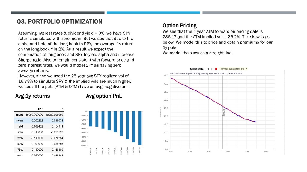
0%, we have SPY returns simulated with zero mean. But we see that due to the alpha and beta of the long book to SPY, the average 1y return on the long book Y is 2%. As a result we expect the combination of long book and SPY to yield alpha and increase Sharpe ratio. Also to remain consistent with forward price and zero interest rates, we would model SPY as having zero average returns. However, since we used the 25 year avg SPY realized vol of 16.78% to simulate SPY & the implied vols are much higher, we see all the puts (ATM & OTM) have an avg. negative pnl. Avg 1y returns Avg option PnL Option Pricing We see that the 1 year ATM forward on pricing date is 286.17 and the ATM implied vol is 26.2%. The skew is as below. We model this to price and obtain premiums for our 1y puts. We model the skew as a straight line.
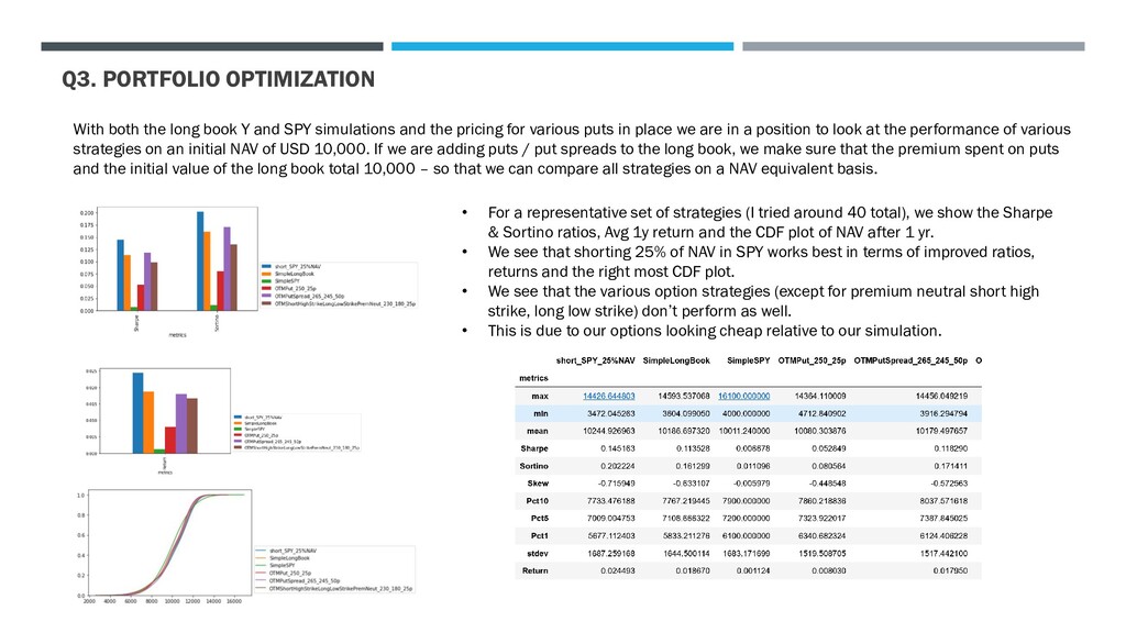
SPY simulations and the pricing for various puts in place we are in a position to look at the performance of various strategies on an initial NAV of USD 10,000. If we are adding puts / put spreads to the long book, we make sure that the premium spent on puts and the initial value of the long book total 10,000 – so that we can compare all strategies on a NAV equivalent basis. • For a representative set of strategies (I tried around 40 total), we show the Sharpe & Sortino ratios, Avg 1y return and the CDF plot of NAV after 1 yr. • We see that shorting 25% of NAV in SPY works best in terms of improved ratios, returns and the right most CDF plot. • We see that the various option strategies (except for premium neutral short high strike, long low strike) don’t perform as well. • This is due to our options looking cheap relative to our simulation.
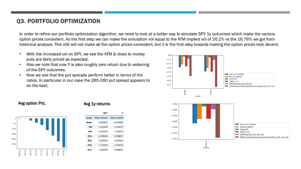
algorithm, we need to look at a better way to simulate SPY 1y outcomes which make the various option prices consistent. As the first step we can make the simulation vol equal to the ATM implied vol of 26.2% vs the 16.78% we got from historical analysis. This still will not make all the option prices consistent, but it is the first step towards making the option prices look decent. Avg option PnL Avg 1y returns • With the increased vol on SPY, we see the ATM & close to money puts are fairly priced as expected. • Also we note that now Y is also roughly zero return due to widening of the SPY outcomes. • Now we see that the put spreads perform better in terms of the ratios. In particular in our case the 285-260 put spread appears to do the best.
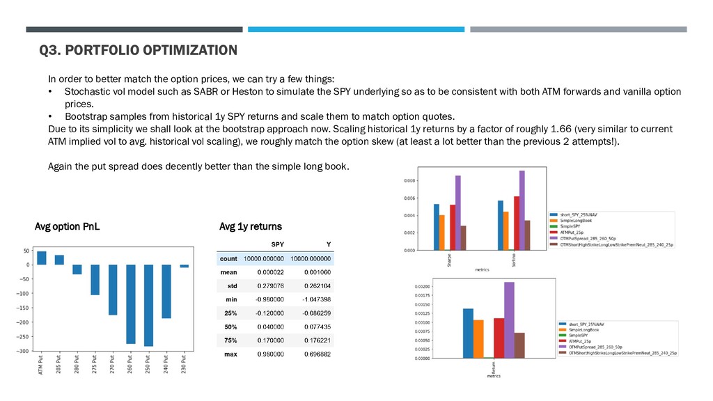
prices, we can try a few things: • Stochastic vol model such as SABR or Heston to simulate the SPY underlying so as to be consistent with both ATM forwards and vanilla option prices. • Bootstrap samples from historical 1y SPY returns and scale them to match option quotes. Due to its simplicity we shall look at the bootstrap approach now. Scaling historical 1y returns by a factor of roughly 1.66 (very similar to current ATM implied vol to avg. historical vol scaling), we roughly match the option skew (at least a lot better than the previous 2 attempts!). Again the put spread does decently better than the simple long book. Avg option PnL Avg 1y returns
to simulate the underlying in a proper way. • As we saw, purely historical vol based simulation might underprice the options traded on a given day, so we might need to use current implied vol levels or a scaled bootstrap or a stochastic vol approach to match the observed skew & the ATM forward. • Bigger question is do we want to simulate the terminal distribution using risk neutral or real world probabilities? • Risk neutral makes sense if the portfolio is dynamically hedged. It can also be argued that since the market is the best predictor of the future (?!) we need to match market quotes. • On the other hand we do know that during times of stress implied vols can spike substantially due to everyone seeking protection at the same time, and therefore significant risk premia could be embedded in the option prices. • So perhaps a judicious combination of both real world & risk neutral aspects might be a better choice. • Purely bootstrapping historically might mean an avg annual return of 10% - this will certainly not be reflected in ATM forwards (due to arbitrage argument). May be keep the historical avg. return but scale the demeaned returns to match option prices? • Once we are comfortable with the simulation process, we can add other features such as optimal weight allocator across different hedge candidates such that the overall portfolio Sharpe or Sortino ratio is maximized. We can also add a penalty term for the number of non zero hedge terms (to minimize transaction cost). A lasso (L1) regularizer might work in this setting.
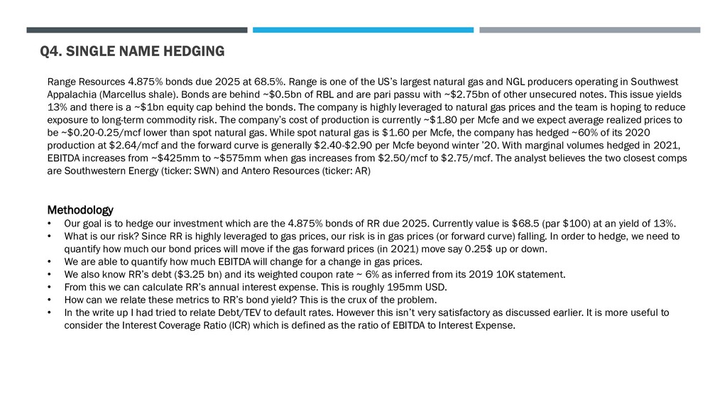
at 68.5%. Range is one of the US’s largest natural gas and NGL producers operating in Southwest Appalachia (Marcellus shale). Bonds are behind ~$0.5bn of RBL and are pari passu with ~$2.75bn of other unsecured notes. This issue yields 13% and there is a ~$1bn equity cap behind the bonds. The company is highly leveraged to natural gas prices and the team is hoping to reduce exposure to long-term commodity risk. The company’s cost of production is currently ~$1.80 per Mcfe and we expect average realized prices to be ~$0.20-0.25/mcf lower than spot natural gas. While spot natural gas is $1.60 per Mcfe, the company has hedged ~60% of its 2020 production at $2.64/mcf and the forward curve is generally $2.40-$2.90 per Mcfe beyond winter ’20. With marginal volumes hedged in 2021, EBITDA increases from ~$425mm to ~$575mm when gas increases from $2.50/mcf to $2.75/mcf. The analyst believes the two closest comps are Southwestern Energy (ticker: SWN) and Antero Resources (ticker: AR) Methodology • Our goal is to hedge our investment which are the 4.875% bonds of RR due 2025. Currently value is $68.5 (par $100) at an yield of 13%. • What is our risk? Since RR is highly leveraged to gas prices, our risk is in gas prices (or forward curve) falling. In order to hedge, we need to quantify how much our bond prices will move if the gas forward prices (in 2021) move say 0.25$ up or down. • We are able to quantify how much EBITDA will change for a change in gas prices. • We also know RR’s debt ($3.25 bn) and its weighted coupon rate ~ 6% as inferred from its 2019 10K statement. • From this we can calculate RR’s annual interest expense. This is roughly 195mm USD. • How can we relate these metrics to RR’s bond yield? This is the crux of the problem. • In the write up I had tried to relate Debt/TEV to default rates. However this isn’t very satisfactory as discussed earlier. It is more useful to consider the Interest Coverage Ratio (ICR) which is defined as the ratio of EBITDA to Interest Expense.
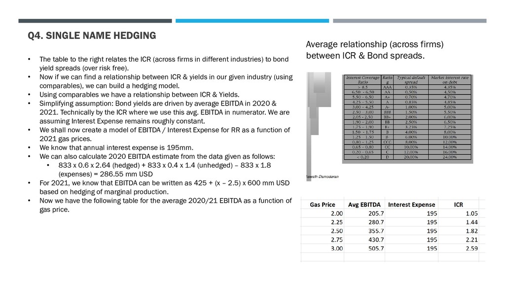
& Bond spreads. • The table to the right relates the ICR (across firms in different industries) to bond yield spreads (over risk free). • Now if we can find a relationship between ICR & yields in our given industry (using comparables), we can build a hedging model. • Using comparables we have a relationship between ICR & Yields. • Simplifying assumption: Bond yields are driven by average EBITDA in 2020 & 2021. Technically by the ICR where we use this avg. EBITDA in numerator. We are assuming Interest Expense remains roughly constant. • We shall now create a model of EBITDA / Interest Expense for RR as a function of 2021 gas prices. • We know that annual interest expense is 195mm. • We can also calculate 2020 EBITDA estimate from the data given as follows: • 833 x 0.6 x 2.64 (hedged) + 833 x 0.4 x 1.4 (unhedged) – 833 x 1.8 (expenses) = 286.55 mm USD • For 2021, we know that EBITDA can be written as 425 + (x – 2.5) x 600 mm USD based on hedging of marginal production. • Now we have the following table for the average 2020/21 EBITDA as a function of gas price.
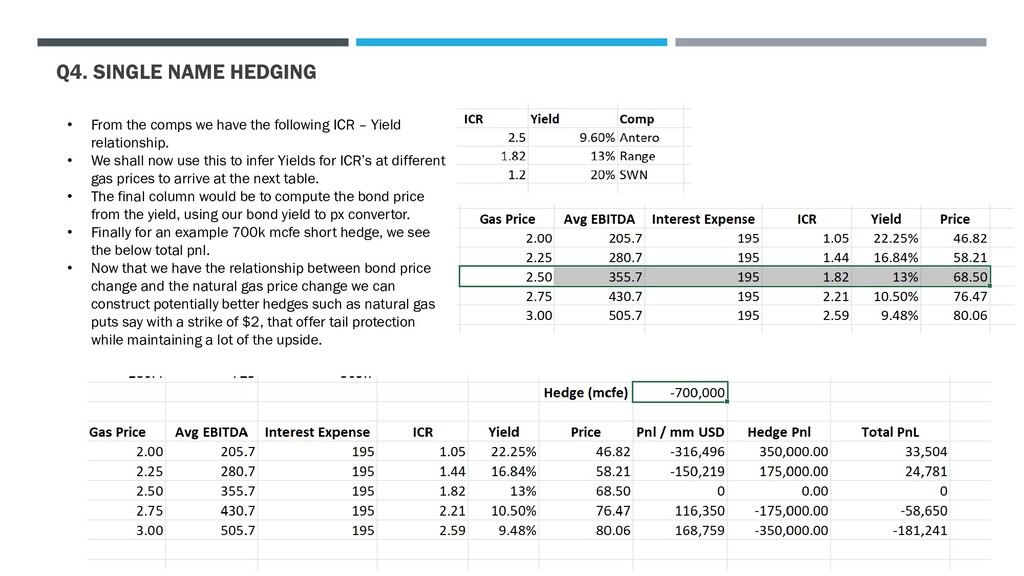
Yield relationship. • We shall now use this to infer Yields for ICR’s at different gas prices to arrive at the next table. • The final column would be to compute the bond price from the yield, using our bond yield to px convertor. • Finally for an example 700k mcfe short hedge, we see the below total pnl. • Now that we have the relationship between bond price change and the natural gas price change we can construct potentially better hedges such as natural gas puts say with a strike of $2, that offer tail protection while maintaining a lot of the upside. Q4. SINGLE NAME HEDGING