one of the most relevant applications of geospatial technology • Millions of dollars are invested in geospatial content (raster data and point clouds) but those data are often not utilized to their full potential • Millions of dollars are invested in geospatial technology that can be used to perform change detection
and mitigate its environmental impacts • Monitor tree canopy loss and focus tree planting efforts • More efficient approach to update your GIS database • Utilizes high resolution ortho imagery • Utilizes elevation data • Perfect application for point cloud data
been historically complex • Readily available true color imagery is not ideal • Elevation data is not accurately co-registered with raster pixels • Need a geospatial expert to perform change detection • Because of the complexities, it is not a realistic possibility for most organizations. • Requires outsourcing
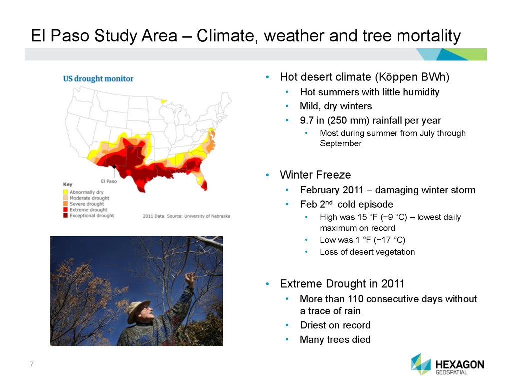
mortality • Hot desert climate (Köppen BWh) • Hot summers with little humidity • Mild, dry winters • 9.7 in (250 mm) rainfall per year • Most during summer from July through September • Winter Freeze • February 2011 – damaging winter storm • Feb 2nd cold episode • High was 15 °F (−9 °C) – lowest daily maximum on record • Low was 1 °F (−17 °C) • Loss of desert vegetation • Extreme Drought in 2011 • More than 110 consecutive days without a trace of rain • Driest on record • Many trees died
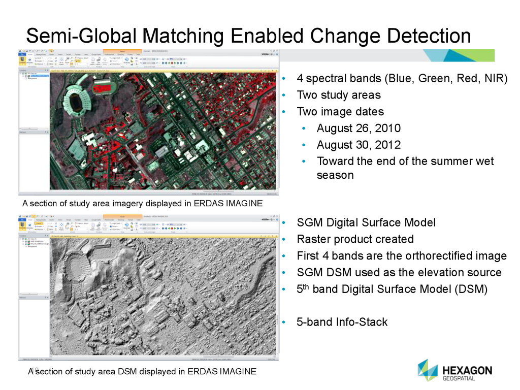
(Blue, Green, Red, NIR) • Two study areas • Two image dates • August 26, 2010 • August 30, 2012 • Toward the end of the summer wet season A section of study area imagery displayed in ERDAS IMAGINE A section of study area DSM displayed in ERDAS IMAGINE • SGM Digital Surface Model • Raster product created • First 4 bands are the orthorectified image • SGM DSM used as the elevation source • 5th band Digital Surface Model (DSM) • 5-band Info-Stack
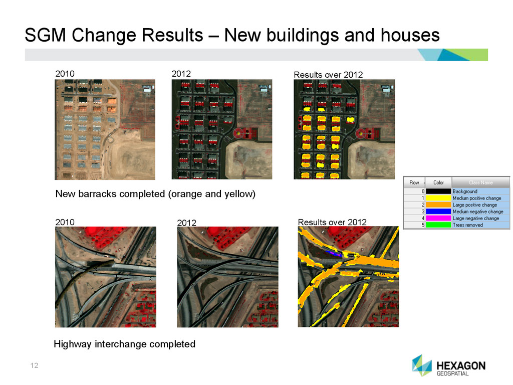
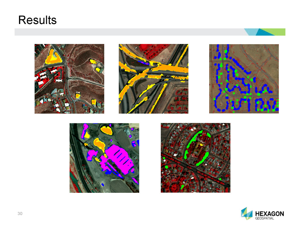
2012 Results over 2012 New commercial building in upper left (orange) and some new houses (yellow and orange) 2010 2012 Results over 2012 Tall commercial buildings have been added (orange)
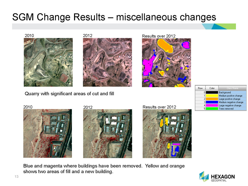
over 2012 Quarry with significant areas of cut and fill 2010 2012 Results over 2012 Blue and magenta where buildings have been removed. Yellow and orange shows two areas of fill and a new building.
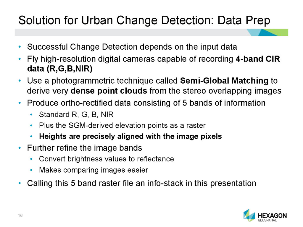
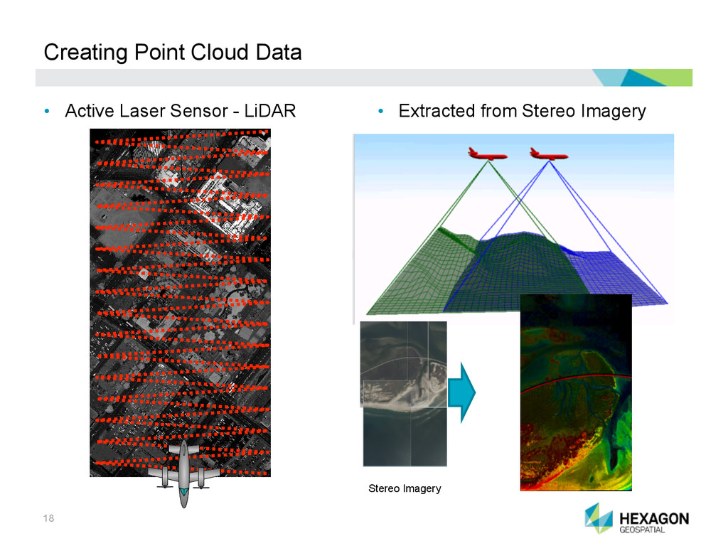
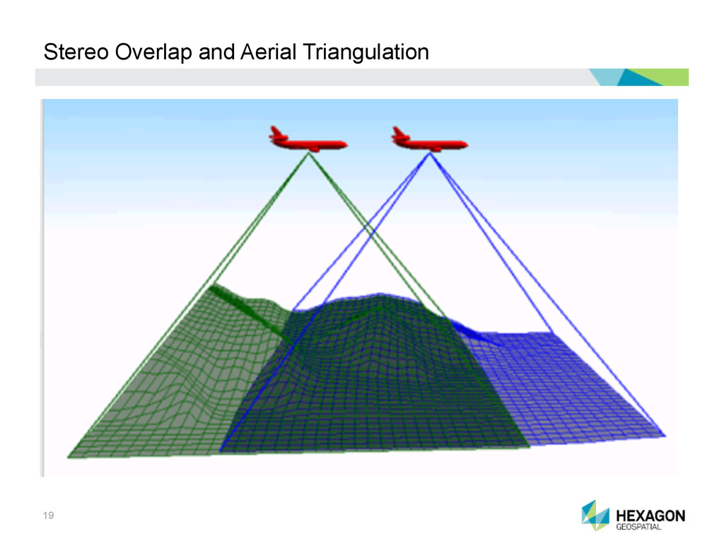
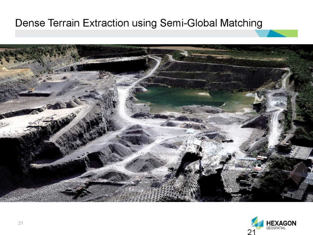
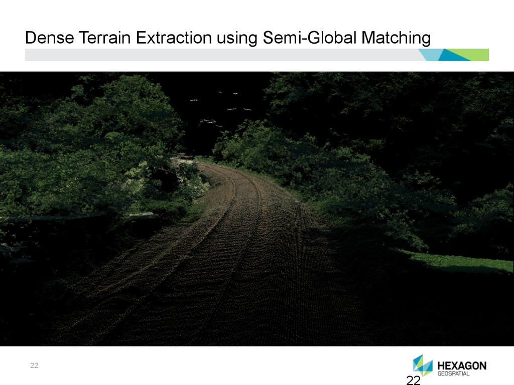
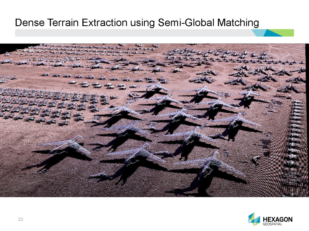
Change Detection depends on the input data • Fly high-resolution digital cameras capable of recording 4-band CIR data (R,G,B,NIR) • Use a photogrammetric technique called Semi-Global Matching to derive very dense point clouds from the stereo overlapping images • Produce ortho-rectified data consisting of 5 bands of information • Standard R, G, B, NIR • Plus the SGM-derived elevation points as a raster • Heights are precisely aligned with the image pixels • Further refine the image bands • Convert brightness values to reflectance • Makes comparing images easier • Calling this 5 band raster file an info-stack in this presentation
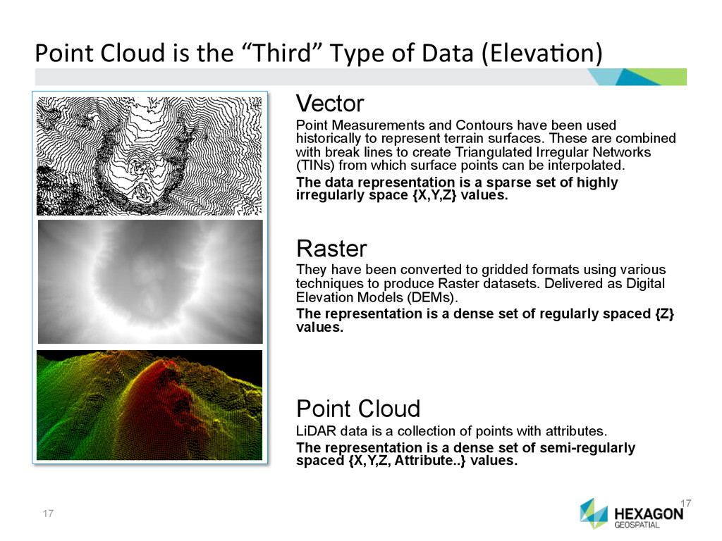
Vector Point Measurements and Contours have been used historically to represent terrain surfaces. These are combined with break lines to create Triangulated Irregular Networks (TINs) from which surface points can be interpolated. The data representation is a sparse set of highly irregularly space {X,Y,Z} values. Raster They have been converted to gridded formats using various techniques to produce Raster datasets. Delivered as Digital Elevation Models (DEMs). The representation is a dense set of regularly spaced {Z} values. Point Cloud LiDAR data is a collection of points with attributes. The representation is a dense set of semi-regularly spaced {X,Y,Z, Attribute..} values. 17
build your own sophisticated, reusable spatial models and save time and money every time the analyst runs the model. • Your resident image analyst creates the model once • Re-usable to your end-users and your customers • Distributable and Repeatable
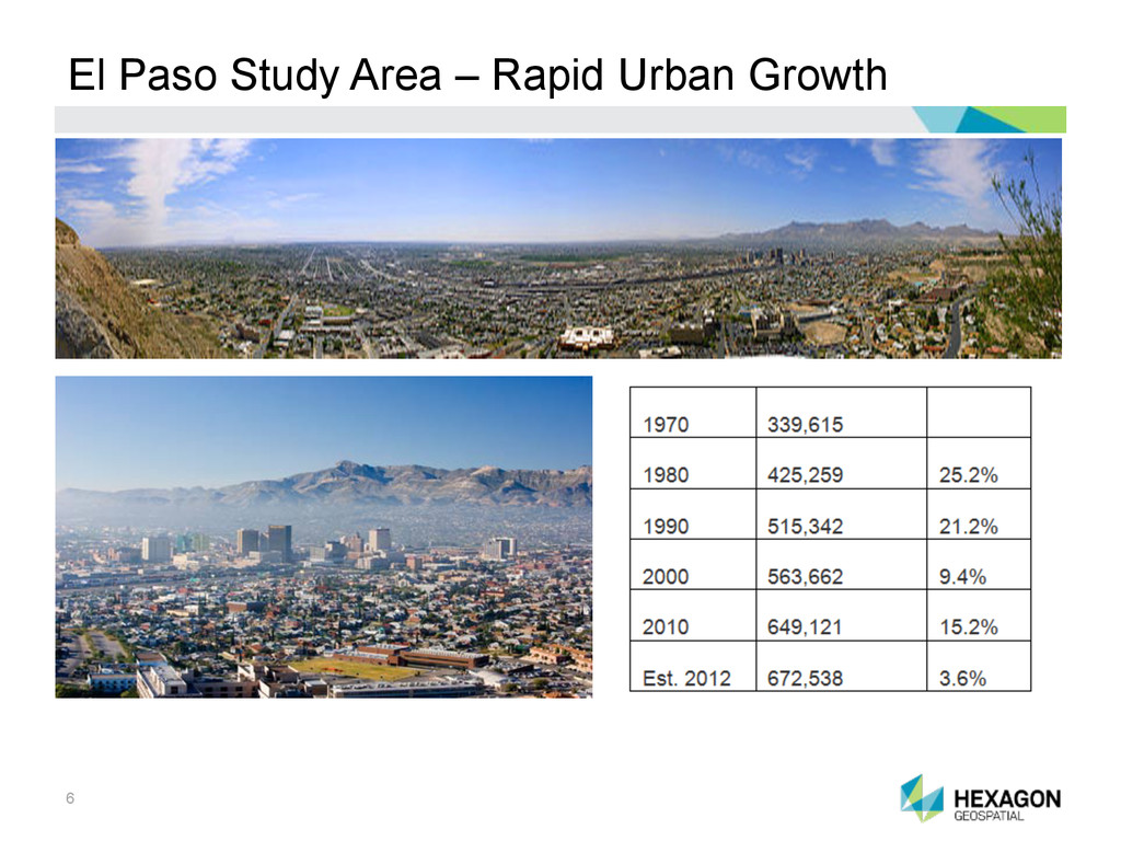
Map urban change • El Paso study area • High growth area • Significant tree mortality • Focus model on changes in buildings and trees • Re-usable • Same model and parameters can be applied to other info-stacks • Ease of use • Minimize input parameters • Provide intelligent default parameters
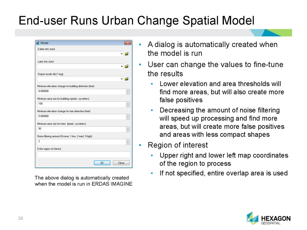
is automatically created when the model is run • User can change the values to fine-tune the results • Lower elevation and area thresholds will find more areas, but will also create more false positives • Decreasing the amount of noise filtering will speed up processing and find more areas, but will create more false positives and areas with less compact shapes • Region of interest • Upper right and lower left map coordinates of the region to process • If not specified, entire overlap area is used The above dialog is automatically created when the model is run in ERDAS IMAGINE
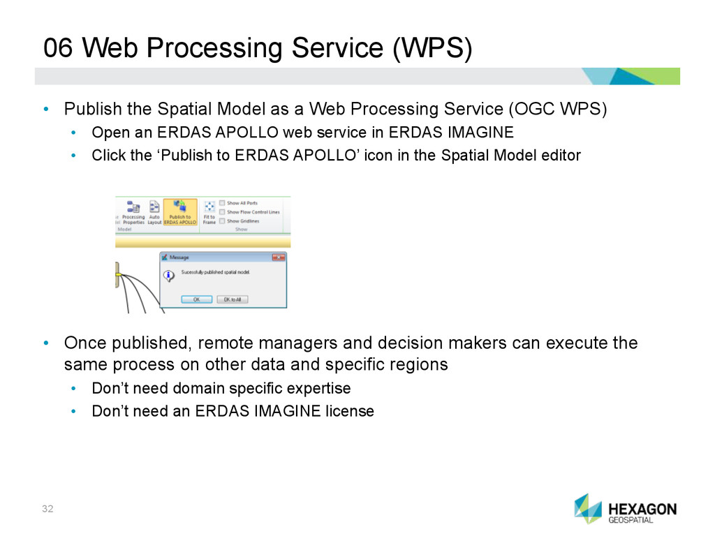
Model as a Web Processing Service (OGC WPS) • Open an ERDAS APOLLO web service in ERDAS IMAGINE • Click the ‘Publish to ERDAS APOLLO’ icon in the Spatial Model editor • Once published, remote managers and decision makers can execute the same process on other data and specific regions • Don’t need domain specific expertise • Don’t need an ERDAS IMAGINE license
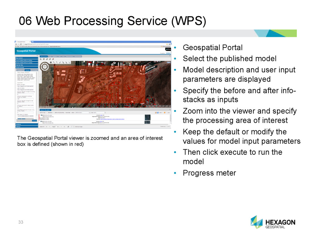
Select the published model • Model description and user input parameters are displayed • Specify the before and after info- stacks as inputs • Zoom into the viewer and specify the processing area of interest • Keep the default or modify the values for model input parameters • Then click execute to run the model • Progress meter The Geospatial Portal viewer is zoomed and an area of interest box is defined (shown in red)
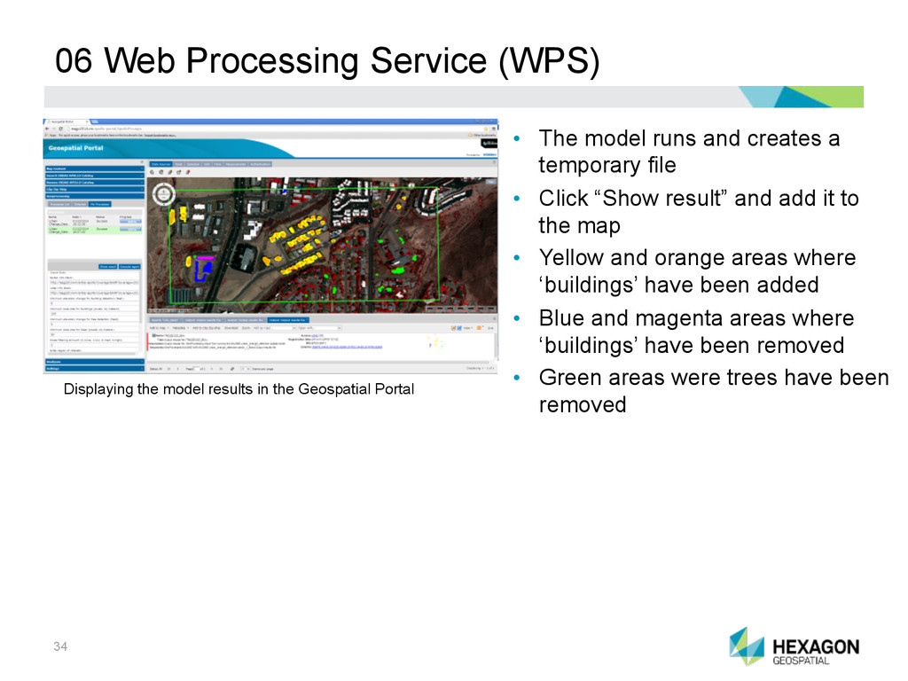
and creates a temporary file • Click “Show result” and add it to the map • Yellow and orange areas where ‘buildings’ have been added • Blue and magenta areas where ‘buildings’ have been removed • Green areas were trees have been removed Displaying the model results in the Geospatial Portal
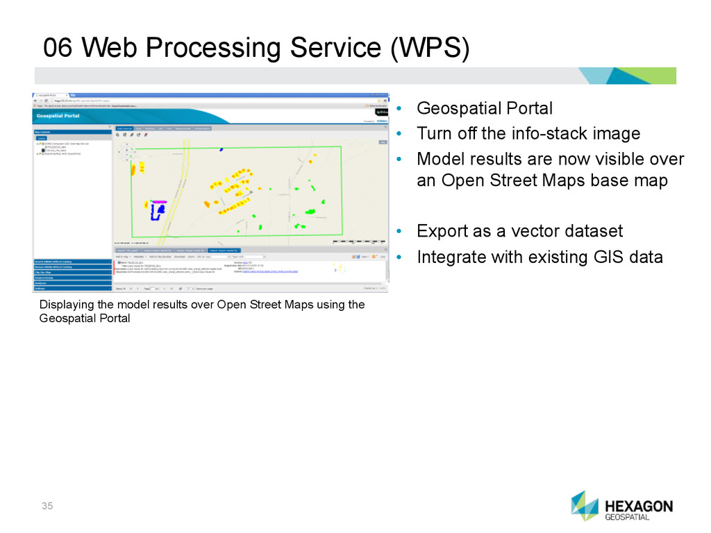
Turn off the info-stack image • Model results are now visible over an Open Street Maps base map • Export as a vector dataset • Integrate with existing GIS data Displaying the model results over Open Street Maps using the Geospatial Portal
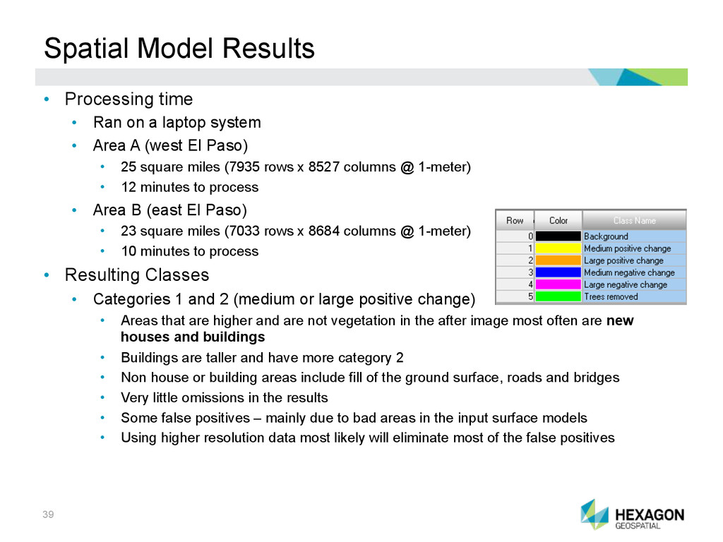
a laptop system • Area A (west El Paso) • 25 square miles (7935 rows x 8527 columns @ 1-meter) • 12 minutes to process • Area B (east El Paso) • 23 square miles (7033 rows x 8684 columns @ 1-meter) • 10 minutes to process • Resulting Classes • Categories 1 and 2 (medium or large positive change) • Areas that are higher and are not vegetation in the after image most often are new houses and buildings • Buildings are taller and have more category 2 • Non house or building areas include fill of the ground surface, roads and bridges • Very little omissions in the results • Some false positives – mainly due to bad areas in the input surface models • Using higher resolution data most likely will eliminate most of the false positives
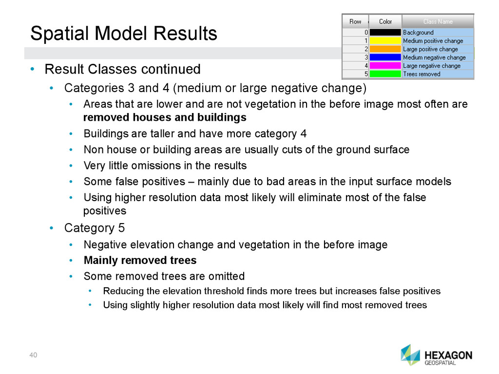
3 and 4 (medium or large negative change) • Areas that are lower and are not vegetation in the before image most often are removed houses and buildings • Buildings are taller and have more category 4 • Non house or building areas are usually cuts of the ground surface • Very little omissions in the results • Some false positives – mainly due to bad areas in the input surface models • Using higher resolution data most likely will eliminate most of the false positives • Category 5 • Negative elevation change and vegetation in the before image • Mainly removed trees • Some removed trees are omitted • Reducing the elevation threshold finds more trees but increases false positives • Using slightly higher resolution data most likely will find most removed trees
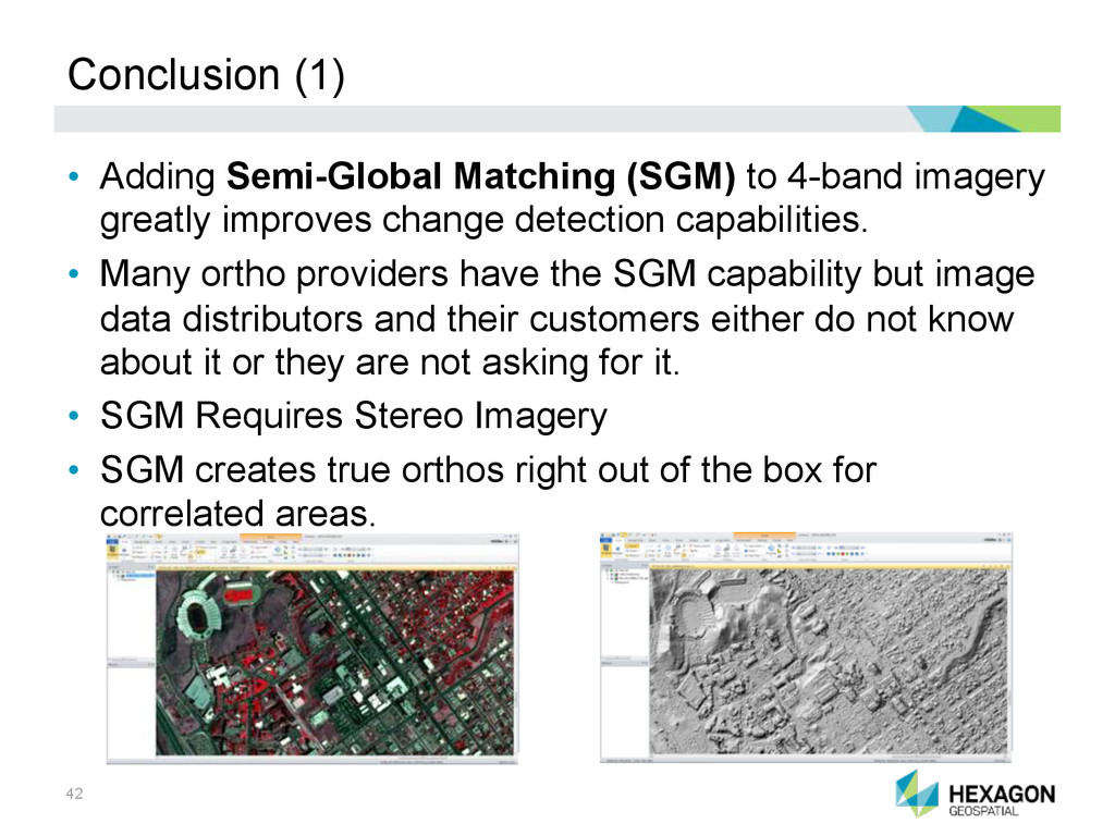
imagery greatly improves change detection capabilities. • Many ortho providers have the SGM capability but image data distributors and their customers either do not know about it or they are not asking for it. • SGM Requires Stereo Imagery • SGM creates true orthos right out of the box for correlated areas.
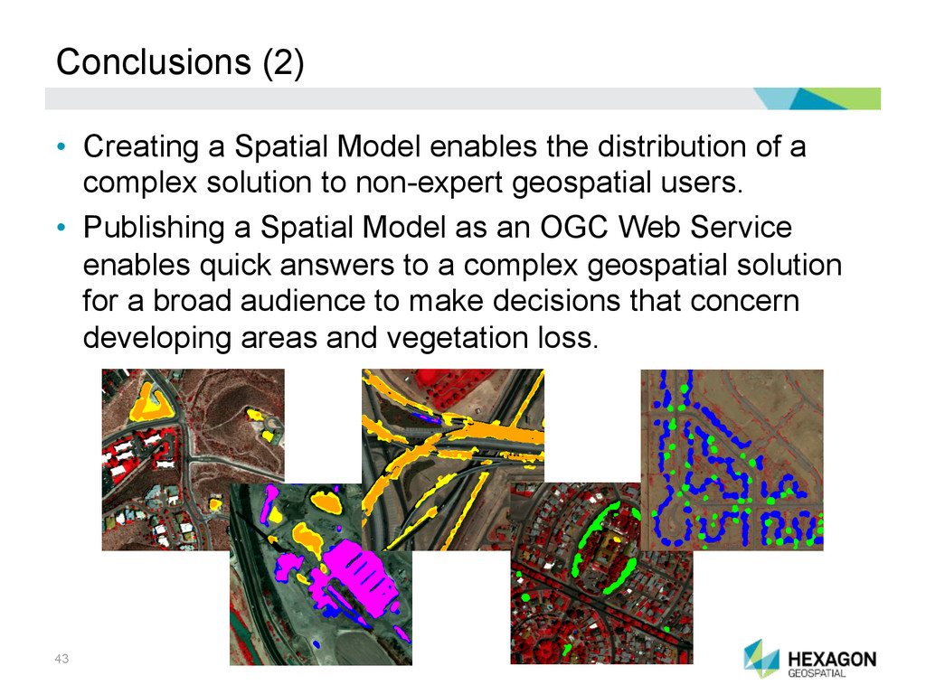
distribution of a complex solution to non-expert geospatial users. • Publishing a Spatial Model as an OGC Web Service enables quick answers to a complex geospatial solution for a broad audience to make decisions that concern developing areas and vegetation loss.