Mapping Milwaukee by Bruce Gorham and Adam Barnes

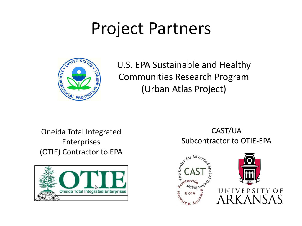
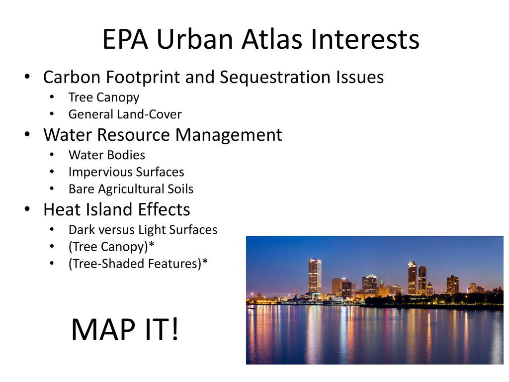
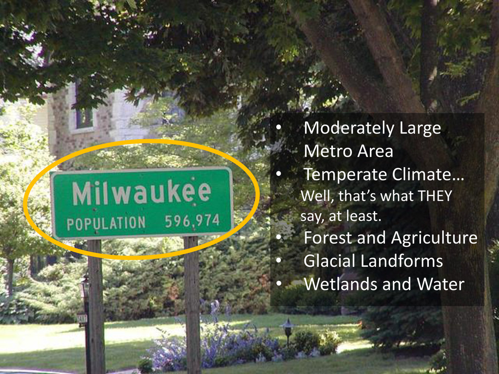
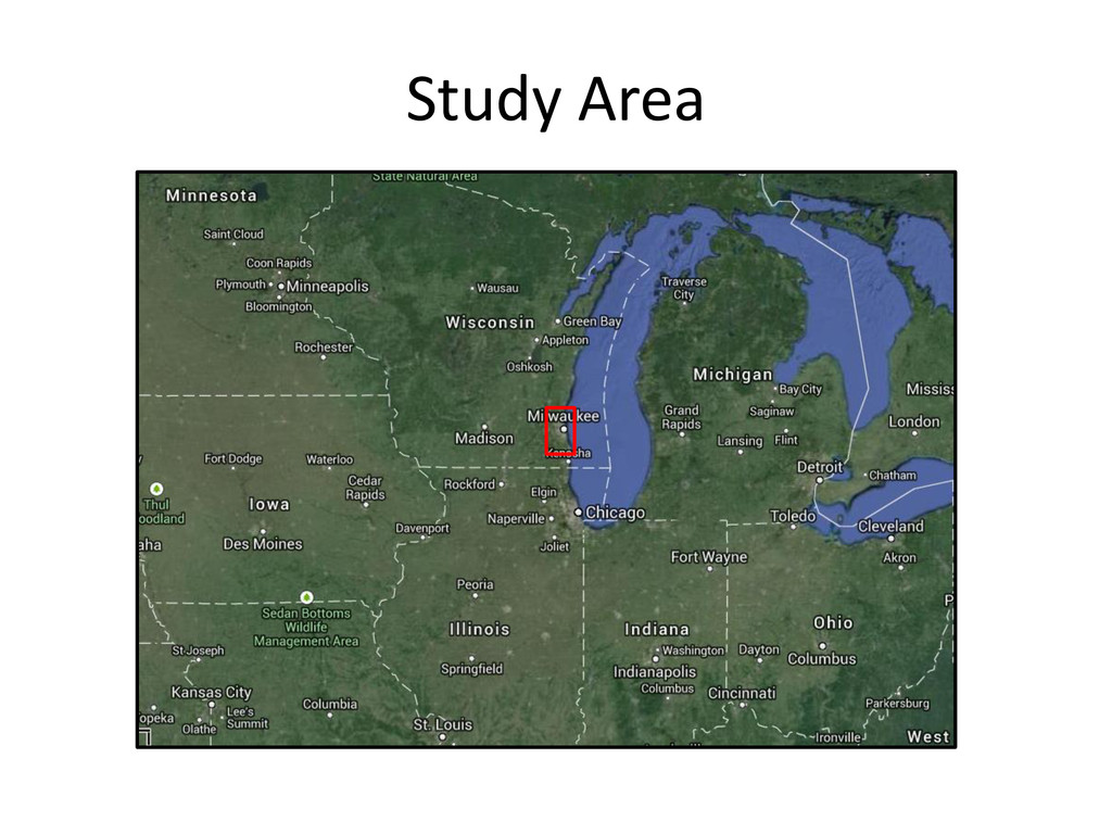
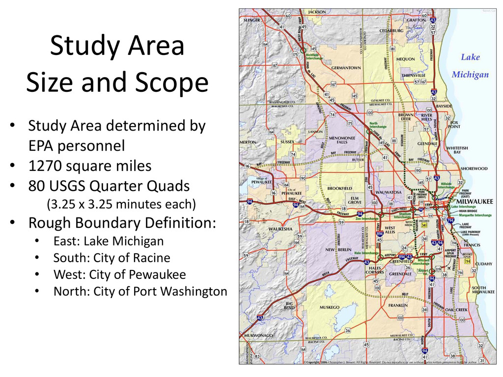
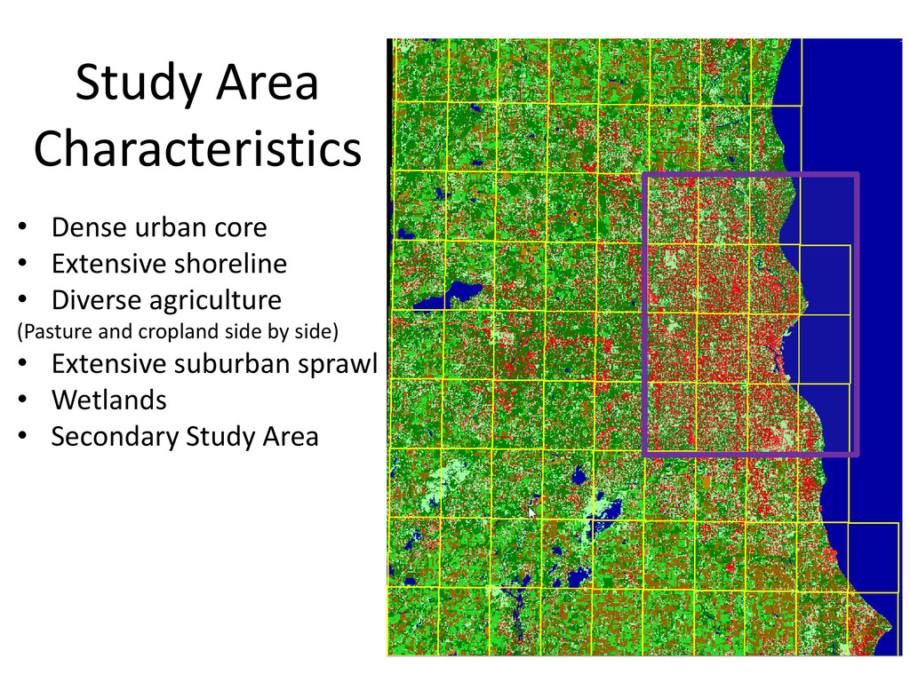
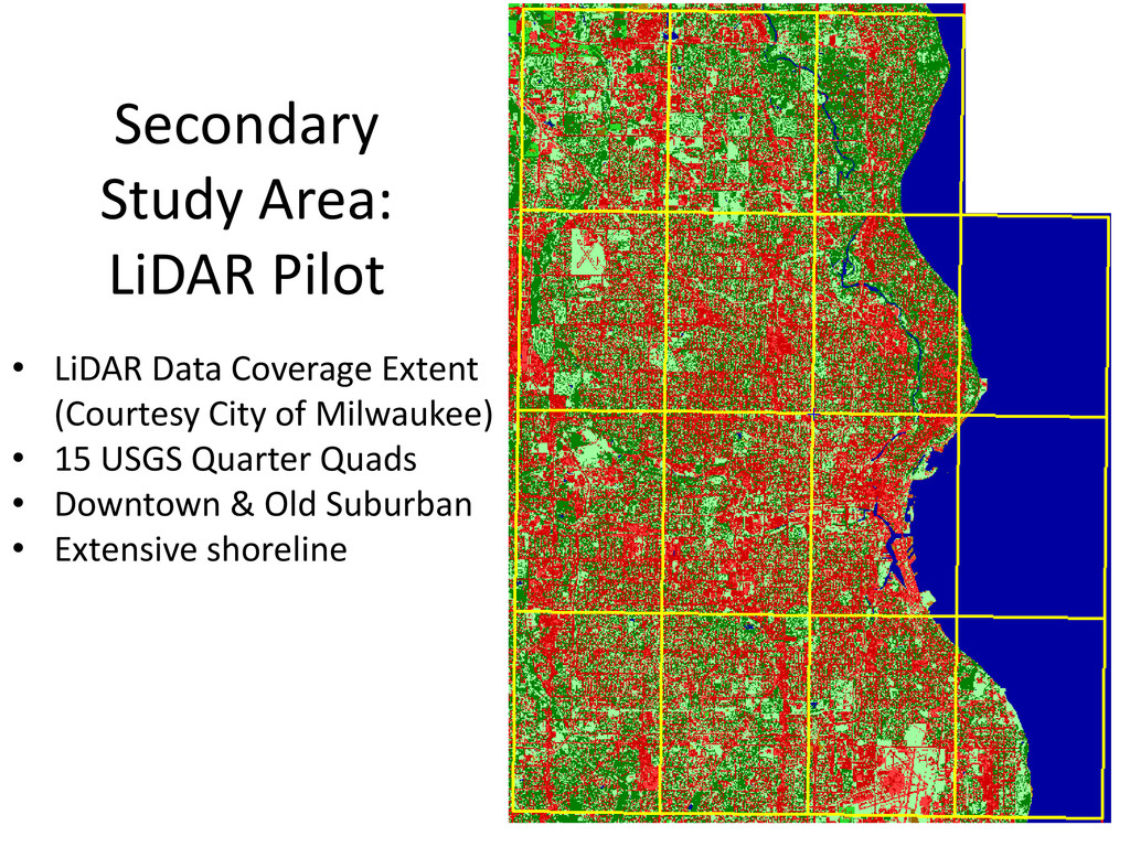
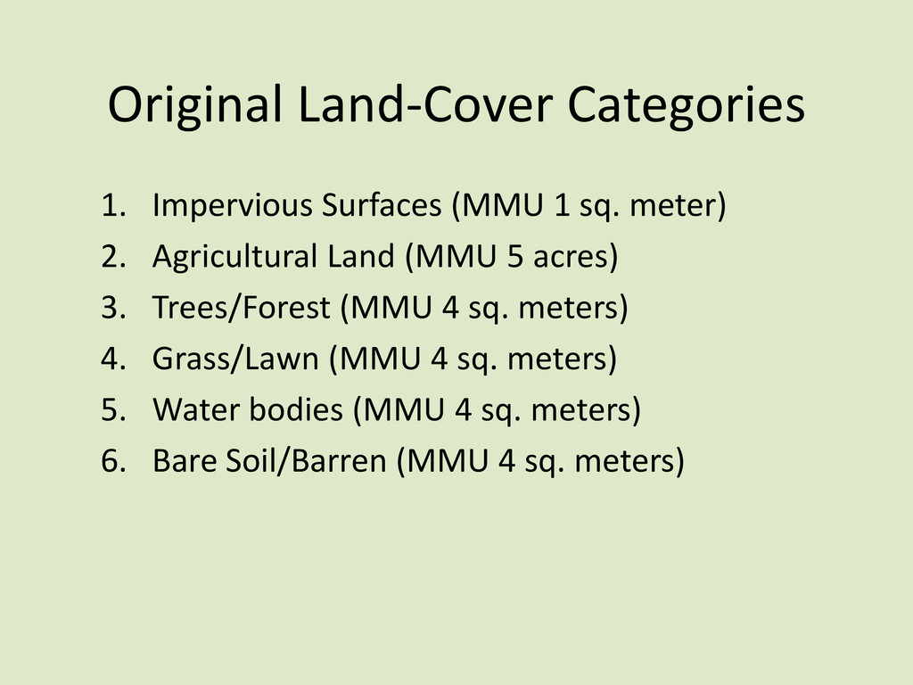
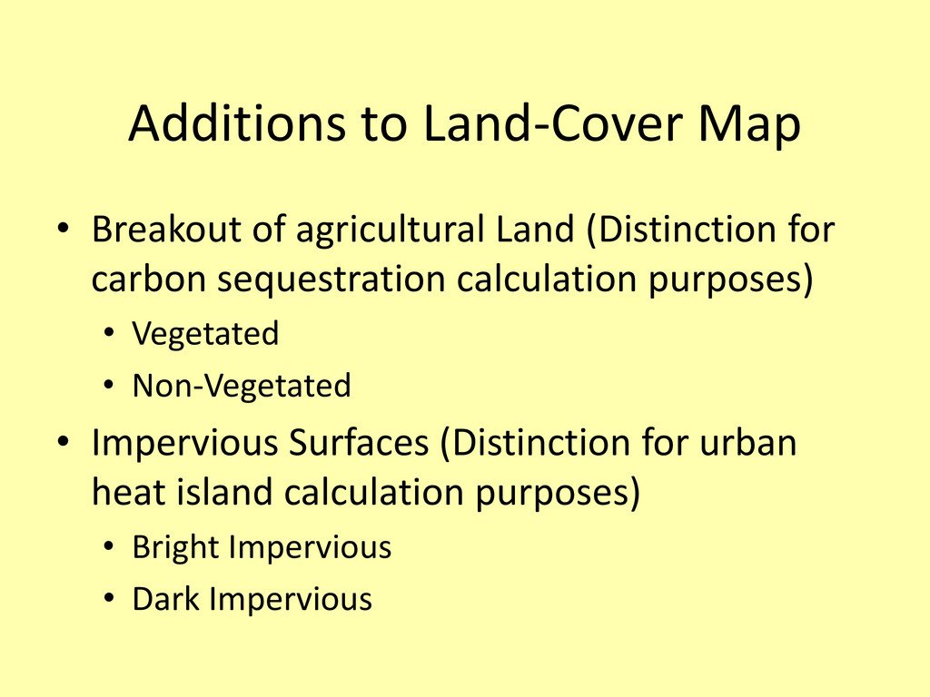
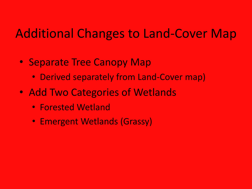
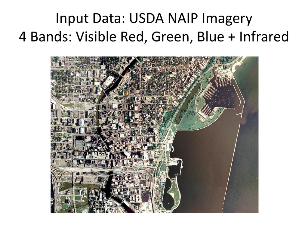
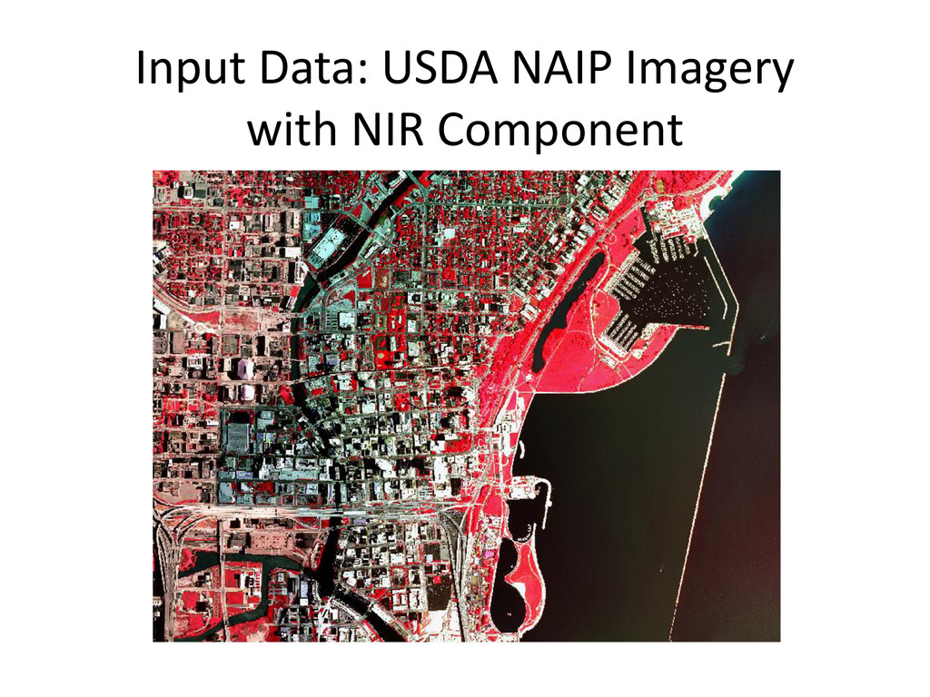
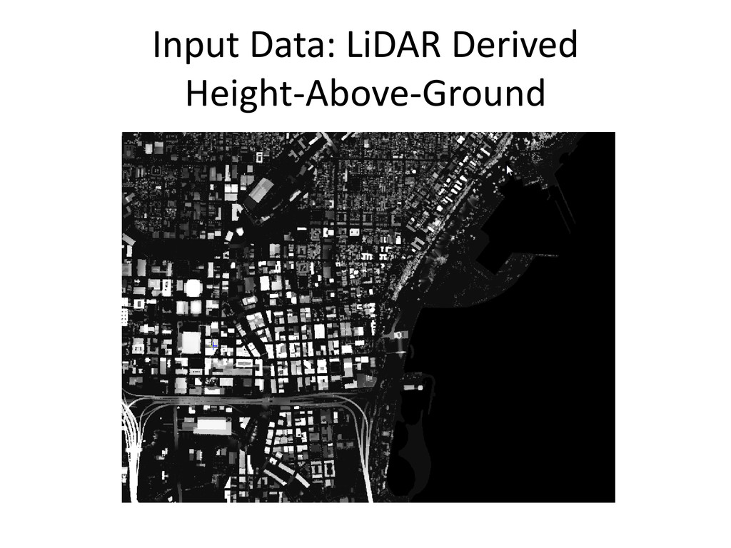
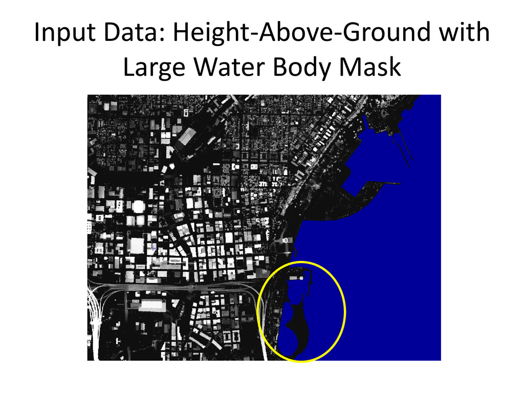
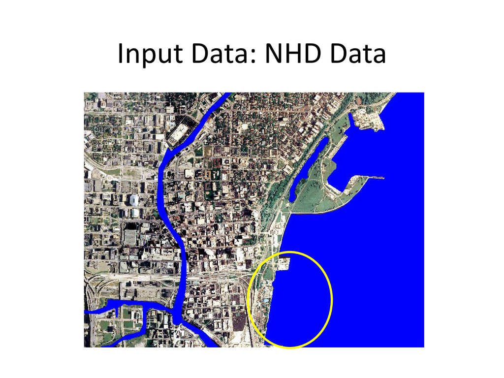
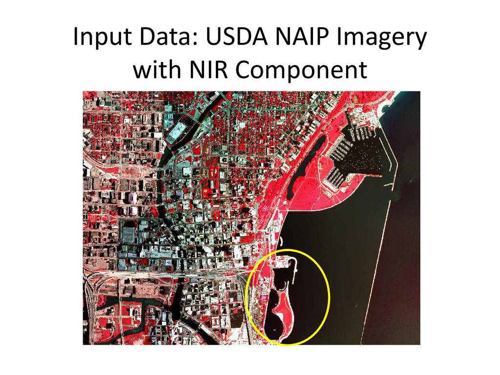
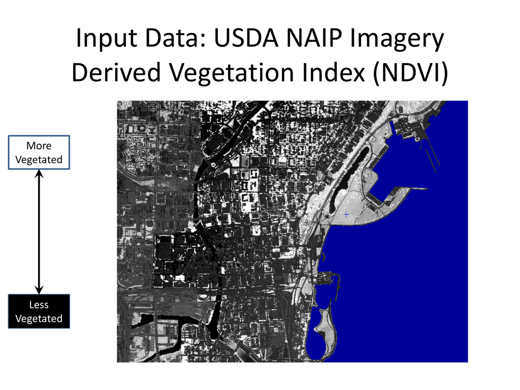
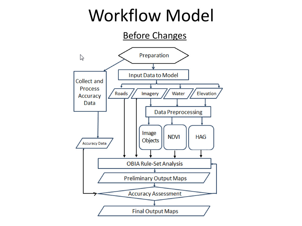
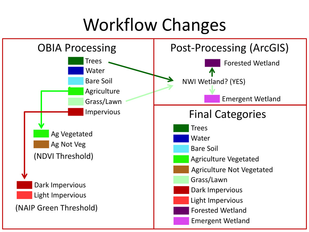
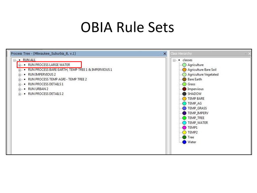
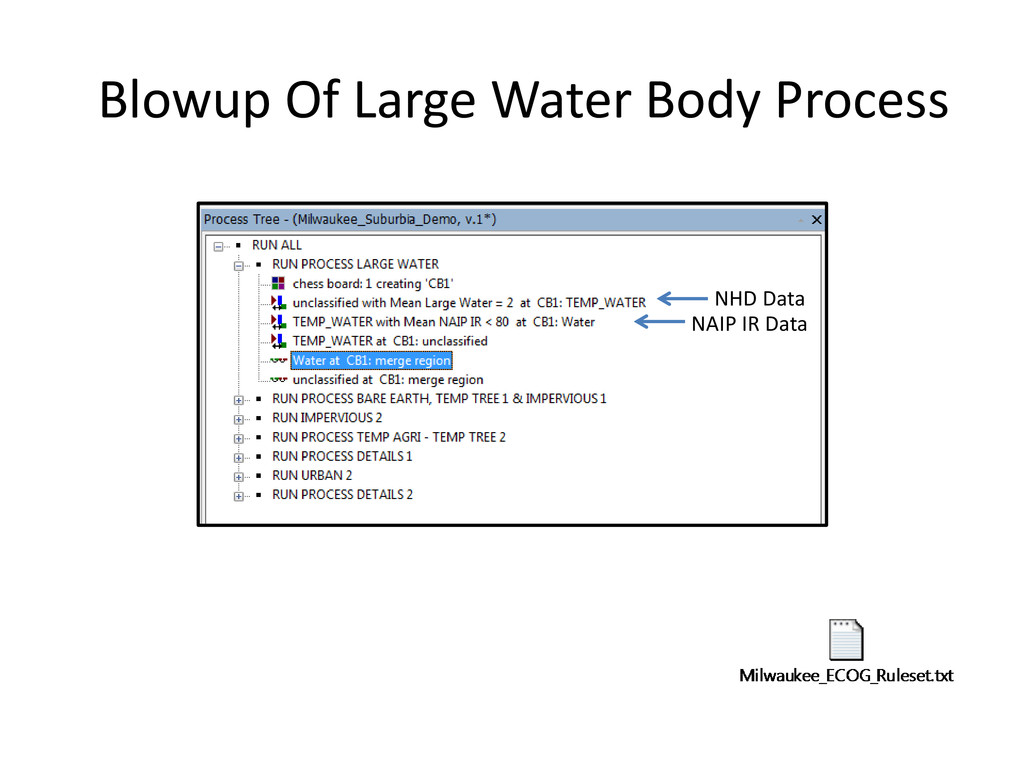
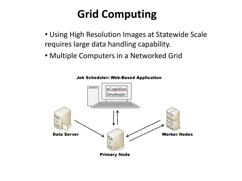
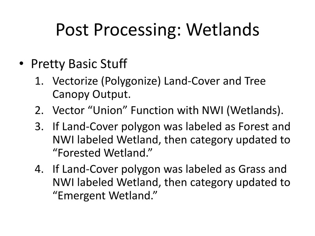
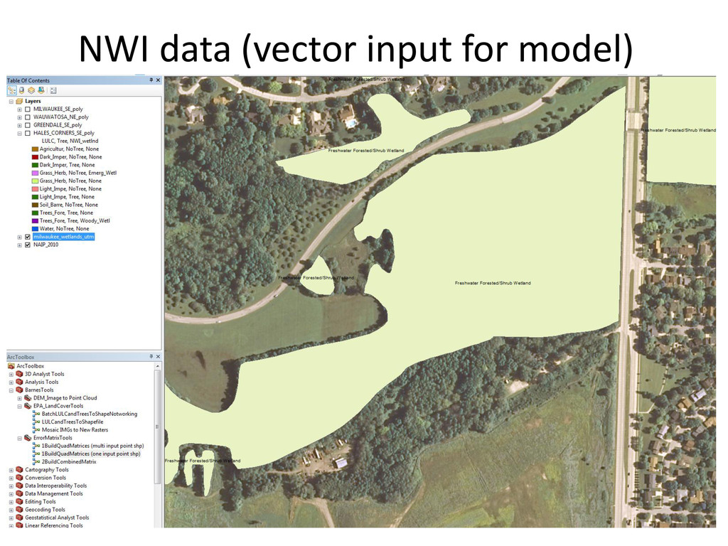
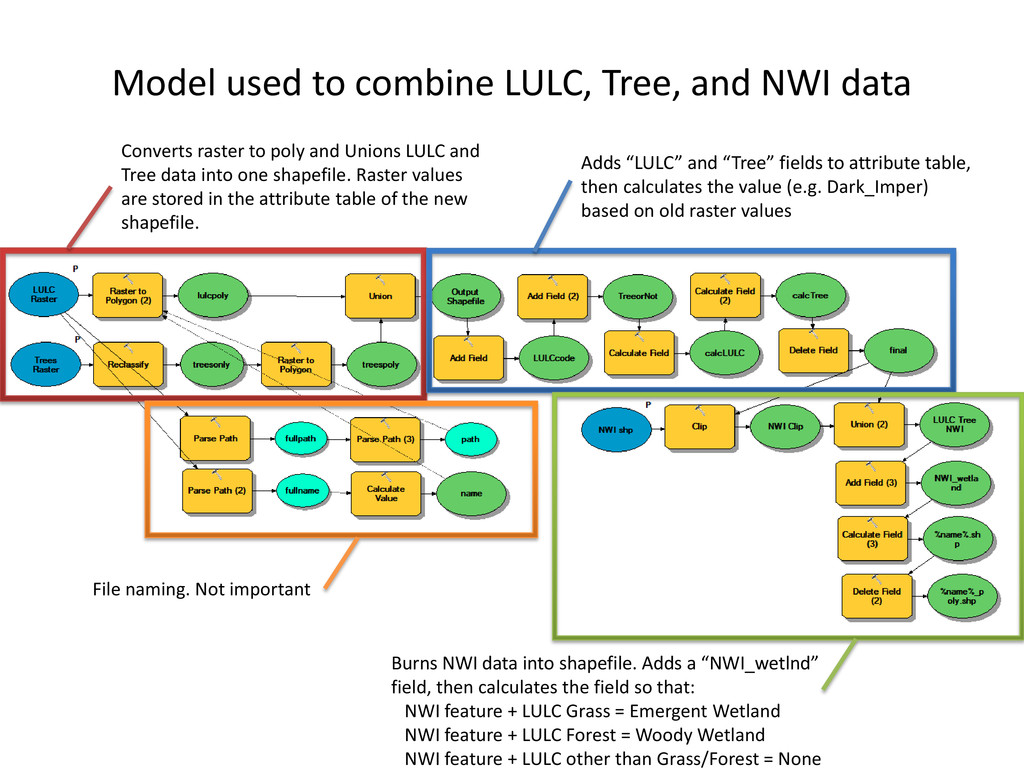
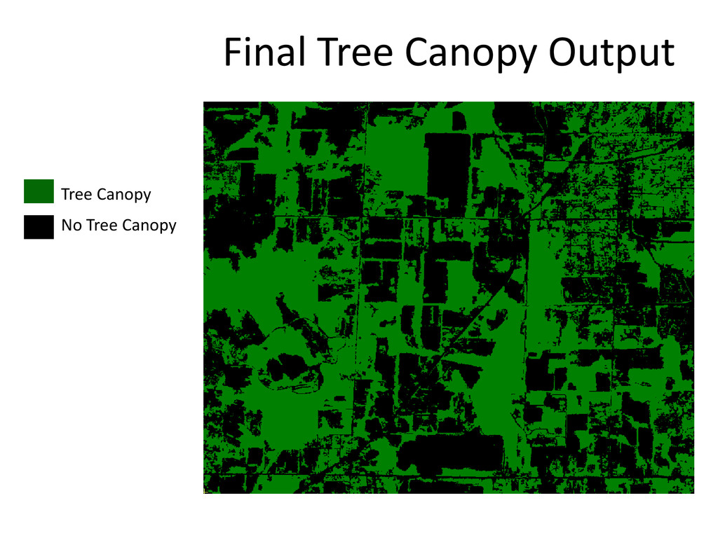
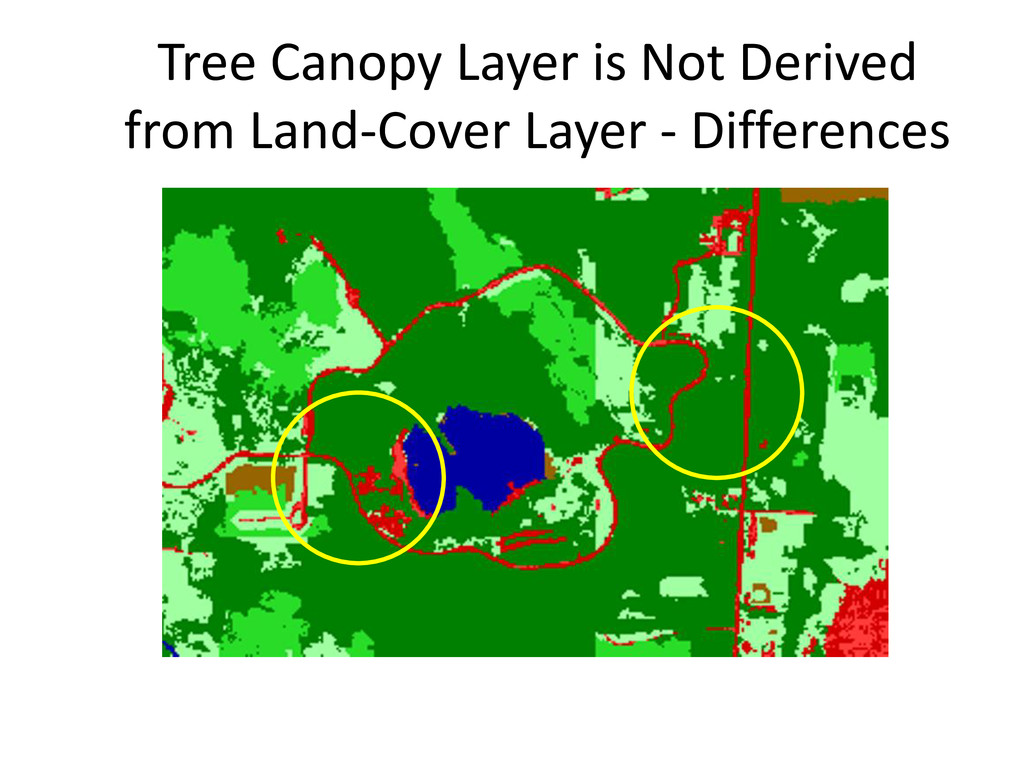
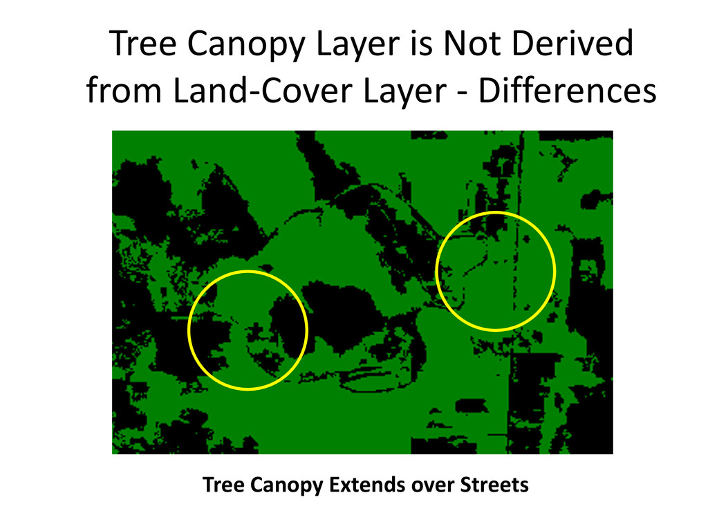
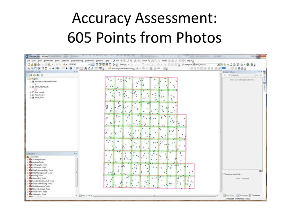
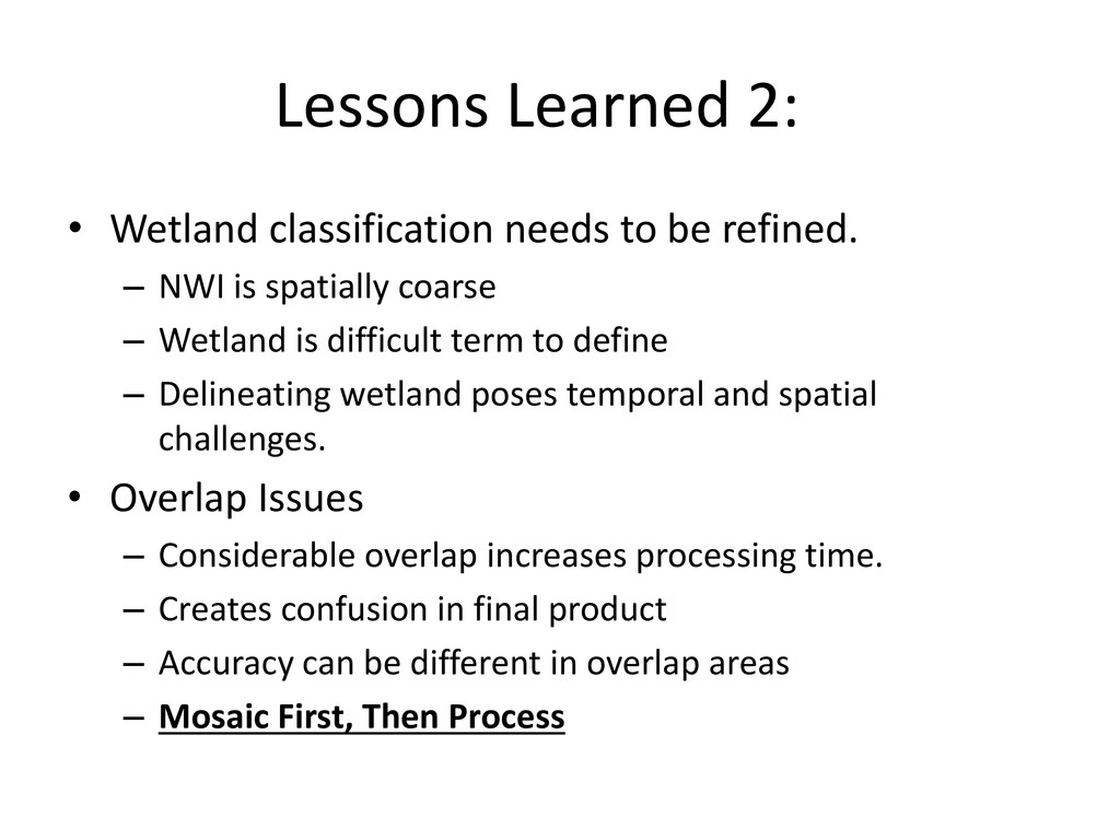
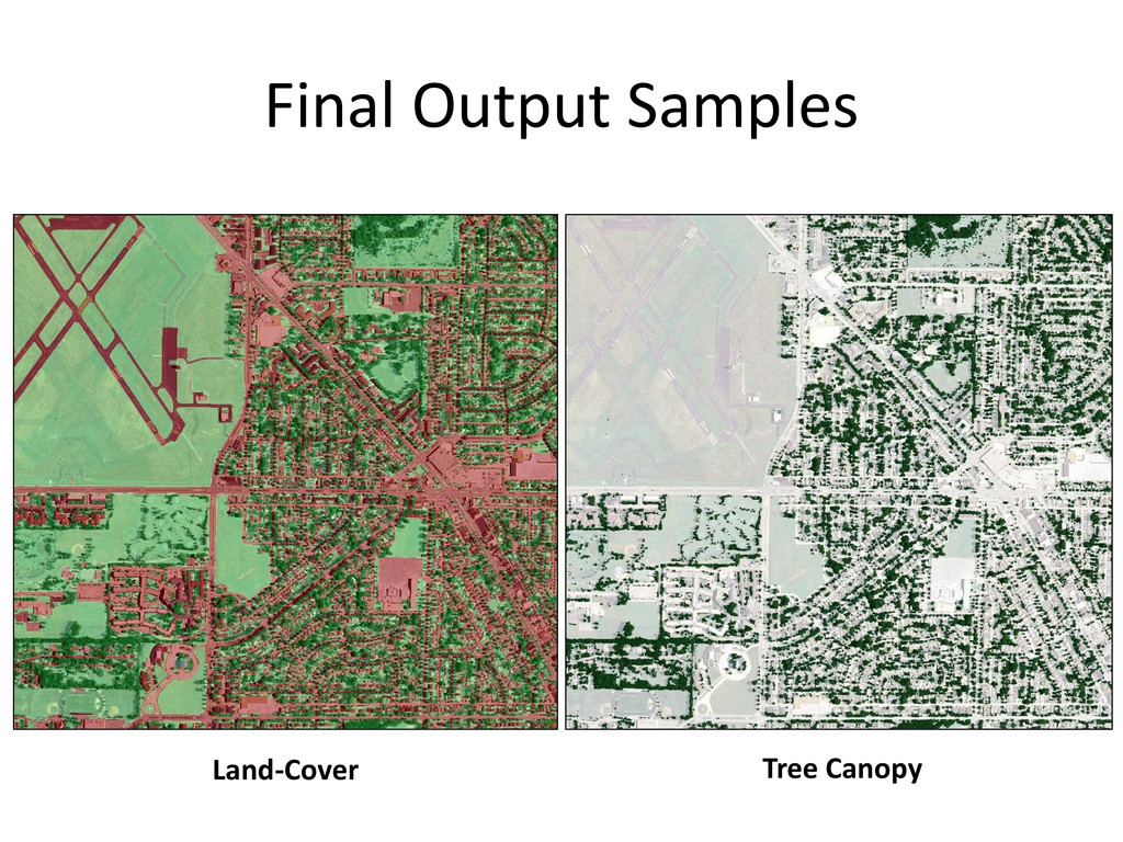
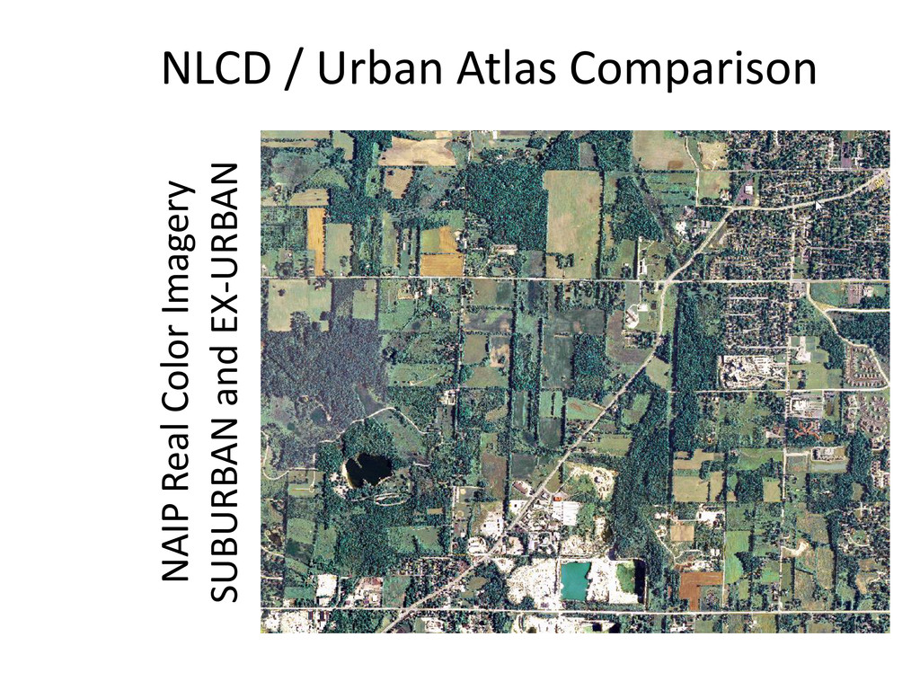
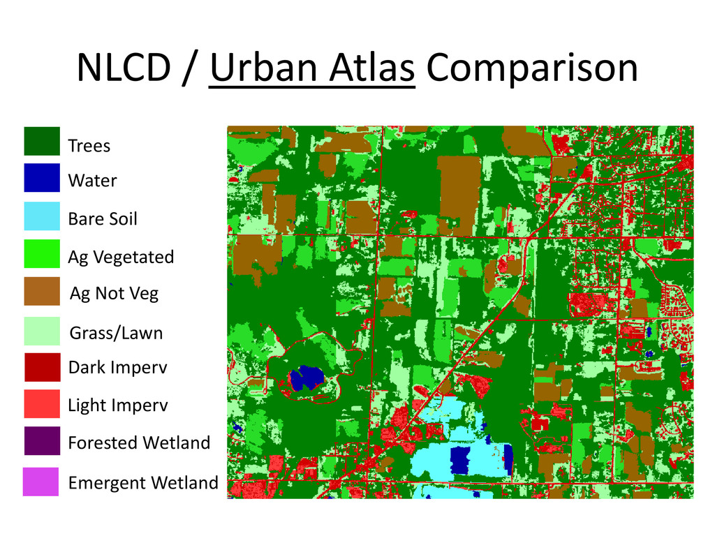
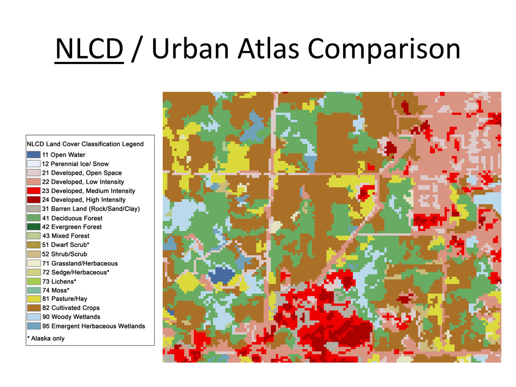
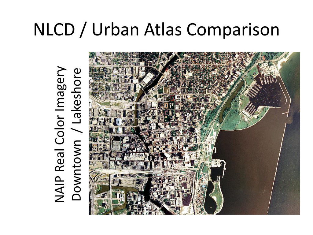
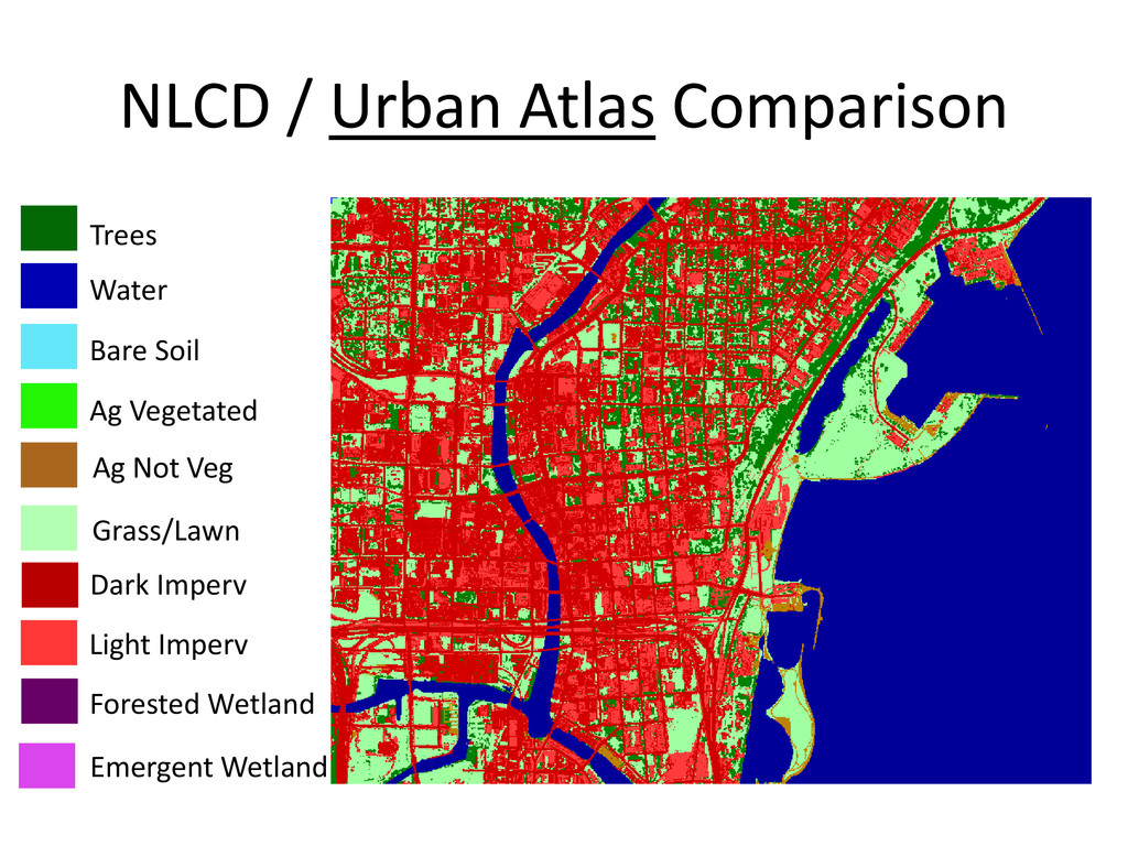
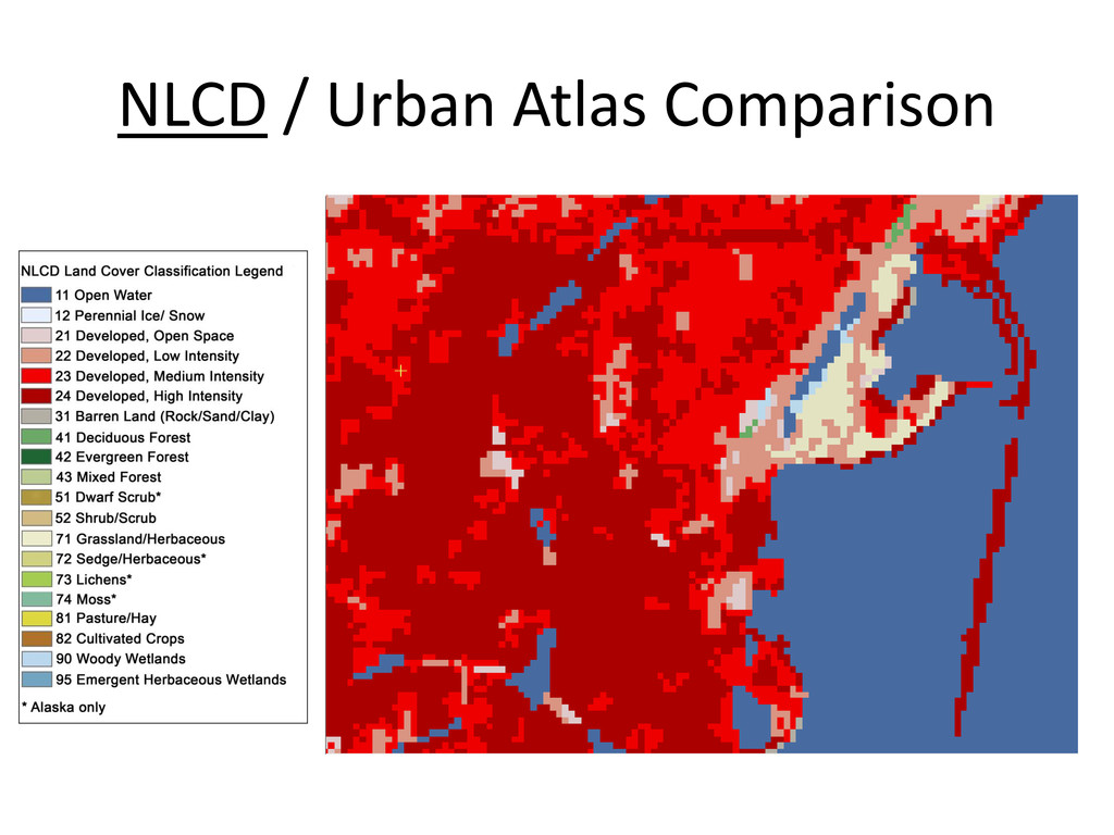
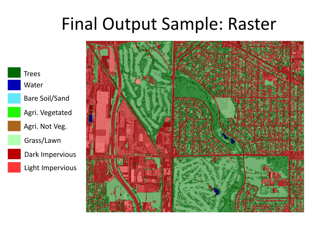
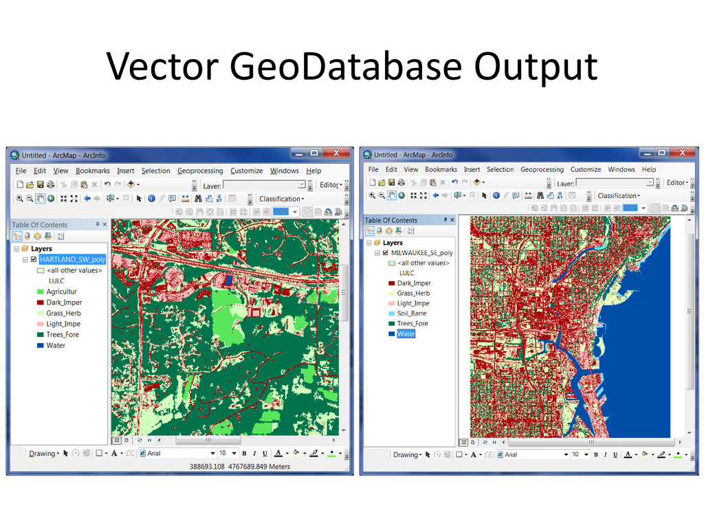
This case study details research and development efforts performed at the Center for Advanced Spatial Technologies for the U.S. Environmental Protection Agency’s Sustainable and Healthy Communities Research Program. The objective of the research presented here was to create spatially and categorically accurate land-cover maps (including tree canopy and impervious surfaces} from 1 meter resolution USDA-NAIP imagery for the Milwaukee, Wisconsin metropolitan area. Secondarily, the project was intended to further the production of consistent, transferable, and automated methods for developing high-resolution impervious surface/land-cover maps and to transfer the resulting methods and technologies to U.S. EPA for use in the mapping of other urban areas. The presentation covers all aspects of the production process: data acquisition and preprocessing, object-based image analysis (ruleset development}, post-processing in ArcGIS, and accuracy assessment. The presentation also addresses the use of ancillary data sets such as LiDAR in the development of quality land-use, land-cover data.

Transcript

1. EPA’s Sustainable and Healthy Communities Research Program (Urban Atlas) Bruce Gorham and Adam Barnes Arkansas GIS User Symposium September 12, 2013 Mapping Milwaukee
2. Project Partners CAST/UA Subcontractor to OTIE-EPA U.S. EPA Sustainable and Healthy Communities Research Program (Urban Atlas Project) Oneida Total Integrated Enterprises (OTIE) Contractor to EPA
3. Project Partners Trimble Imaging Innovation Program TIP PCI Geomatics Educational Alliance Program Advanced Imaging Software Object-Based Image Analysis Software
4. … and our Milwaukee Partners. Just kidding folks.
5. EPA Urban Atlas Interests • Carbon Footprint and Sequestration Issues • Tree Canopy • General Land-Cover • Water Resource Management • Water Bodies • Impervious Surfaces • Bare Agricultural Soils • Heat Island Effects • Dark versus Light Surfaces • (Tree Canopy)* • (Tree-Shaded Features)* MAP IT!
6. • Moderately Large Metro Area • Temperate Climate… Well, that’s what THEY say, at least. • Forest and Agriculture • Glacial Landforms • Wetlands and Water
7. Study Area
8. Study Area Size and Scope • Study Area determined by EPA personnel • 1270 square miles • 80 USGS Quarter Quads (3.25 x 3.25 minutes each) • Rough Boundary Definition: • East: Lake Michigan • South: City of Racine • West: City of Pewaukee • North: City of Port Washington
9. Study Area Characteristics • Dense urban core • Extensive shoreline • Diverse agriculture (Pasture and cropland side by side) • Extensive suburban sprawl • Wetlands • Secondary Study Area
10. Secondary Study Area: LiDAR Pilot • LiDAR Data Coverage Extent (Courtesy City of Milwaukee) • 15 USGS Quarter Quads • Downtown & Old Suburban • Extensive shoreline
11. Project Specifications • One meter resolution land-cover map • Source data: only nationally available • Object-oriented processing methods • Workflow must be portable (as much as possible)
12. Original Land-Cover Categories 1. Impervious Surfaces (MMU 1 sq. meter) 2. Agricultural Land (MMU 5 acres) 3. Trees/Forest (MMU 4 sq. meters) 4. Grass/Lawn (MMU 4 sq. meters) 5. Water bodies (MMU 4 sq. meters) 6. Bare Soil/Barren (MMU 4 sq. meters)
13. Additions to Land-Cover Map • Breakout of agricultural Land (Distinction for carbon sequestration calculation purposes) • Vegetated • Non-Vegetated • Impervious Surfaces (Distinction for urban heat island calculation purposes) • Bright Impervious • Dark Impervious
14. Added Pilot Study • LiDAR pilot study • Covered 15 QQs of Central Milwaukee • Required the development of entirely separate workflow (OBIA rule set) • Required me to learn how to use eCognition LiDAR processing tools (What’s that they say about old dogs and new tricks?)
15. Additional Changes to Land-Cover Map • Separate Tree Canopy Map • Derived separately from Land-Cover map) • Add Two Categories of Wetlands • Forested Wetland • Emergent Wetlands (Grassy)
16. Input Data: USDA NAIP Imagery 4 Bands: Visible Red, Green, Blue + Infrared
17. Input Data: USDA NAIP Imagery with NIR Component
18. Input Data: LiDAR Derived Height-Above-Ground
19. Input Data: Height-Above-Ground with Large Water Body Mask
20. Input Data: NHD Data
21. Input Data: USDA NAIP Imagery with NIR Component
22. Input Data: NHD Data
23. Input Data: USDA NAIP Imagery Derived Vegetation Index (NDVI) More Vegetated Less Vegetated
24. Other Input Datasets • Eventually Used – Railroads - Added Later EPA Request – NWI Wetlands (Employed in Post Processing) Added Later EPA Request • Not Used (Mostly because we are seeking a repeatable methodology.) – Downtown parcel polygons (inconsistent) – Downtown double-sided roads (inconsistent) – Downtown land-use polygons (inconsistent and spatial inaccuracies)
25. Object-Based Image Analysis 3. Define classification parameters based on hundreds of predefined and user-defined object attributes. 4. Apply classification parameters. 1. Create image objects from raster and vector input data. (Segmentation) 2. Reshape image objects by splitting, merging, growing, shrinking based on object and/or pixel attributes. Most Time Consuming Tasks
26. Workflow Model Before Changes
27. Workflow Changes Bare Soil Trees Agriculture Water Grass/Lawn Impervious Ag Not Veg Ag Vegetated Dark Impervious Light Impervious (NDVI Threshold) (NAIP Green Threshold) Post-Processing (ArcGIS) Forested Wetland Emergent Wetland OBIA Processing NWI Wetland? (YES) Bare Soil Trees Water Agriculture Not Vegetated Agriculture Vegetated Grass/Lawn Dark Impervious Light Impervious Forested Wetland Emergent Wetland Final Categories
28. OBIA Rule Sets
29. Blowup Of Large Water Body Process NHD Data NAIP IR Data
30. Grid Computing • Using High Resolution Images at Statewide Scale requires large data handling capability. • Multiple Computers in a Networked Grid Job Scheduler: Web-Based Application Data Server Primary Node Worker Nodes
31. Post Processing: Wetlands • Pretty Basic Stuff 1. Vectorize (Polygonize) Land-Cover and Tree Canopy Output. 2. Vector “Union” Function with NWI (Wetlands). 3. If Land-Cover polygon was labeled as Forest and NWI labeled Wetland, then category updated to “Forested Wetland.” 4. If Land-Cover polygon was labeled as Grass and NWI labeled Wetland, then category updated to “Emergent Wetland.”
32. NWI data (vector input for model)
33. LULC / Tree / NWI categories Dark_Imper/Tree/None Dark_Imper/NoTree/None Trees_Fore/Tree/Woody_Wetl Grass_Herb/NoTree/Emerg_Wetl
34. Model used to combine LULC, Tree, and NWI data Converts raster to poly and Unions LULC and Tree data into one shapefile. Raster values are stored in the attribute table of the new shapefile. Adds “LULC” and “Tree” fields to attribute table, then calculates the value (e.g. Dark_Imper) based on old raster values File naming. Not important Burns NWI data into shapefile. Adds a “NWI_wetlnd” field, then calculates the field so that: NWI feature + LULC Grass = Emergent Wetland NWI feature + LULC Forest = Woody Wetland NWI feature + LULC other than Grass/Forest = None
35. Final Tree Canopy Output Tree Canopy No Tree Canopy
36. Tree Canopy Layer is Not Derived from Land-Cover Layer - Differences
37. Tree Canopy Layer is Not Derived from Land-Cover Layer - Differences Tree Canopy Extends over Streets
38. Accuracy Assessment: 605 Points from Photos
39. Accuracy Assessment: Categorical Adjustment We added assessment points for specific categories: 1. In order for each category to have at least 50 points. 2. In order to match the spatial coverage: (i.e. if 33% of the mapped land-cover was forest then approximately 33% of the accuracy assessment points should be in the forest category.)
40. Accuracy Assessment: All Points Reflects differences between Field Sampling and Random Point Sampling
41. Accuracy Assessment: Point Quality Point Quality Assessment Criteria: 1. Interpreter Confidence Level (20%, 40%, 60%, 80%, 100%) 2. Is point on border between two or more categories? (Yes, No) 3. Is point in shadowed area? (Yes, No) 1. 100% Confidence 2. Border? No 3. Shadowed? No 1. 80% Confidence 2. Border? Yes 3. Shadowed? No 1. 40% Confidence 2. Border? Yes 3. Shadowed? Yes
42. Accuracy Assessment with Point Quality/Confidence Only Points with Confidence > 80%, not on boundary, not in shadow
43. Accuracy Assessment of LiDAR Areas with Point Quality/Confidence Only Points with Confidence > 80%, not on boundary, not in shadow Notes: Some categorical errors worsened by post processing changes in classification scheme. 1. Aglands split into vegetated/non-vegetated fields. (Bare Soil Confusion) 2. The eventual separation of LULC and Tree Canopy layers also caused accuracy assessment difficulties.
44. Comparison: LiDAR H-A-G vs. No LiDAR • With LiDAR better distinction between tree and other vegetation types. • With LiDAR better delineation of most features falling in shadow. • Without LiDAR no errors associated with spatial misalignment • Without LiDAR faster/easier ruleset development • LiDAR not available in all places, no consistency issues. • LiDAR datasets are not standardized from place to place. Consistency.
45. Addressing Spectral Differences within and between NAIP Quarter Quads • Rely more on spectral indices such as NDVI. • Rely more on IR values which are less influenced by varying atmospheric conditions. • Considerable reliance on texture characteristics such as “homogeneity” and “contrast.” • Use of spatial characteristics such as object size, shape, and proximity to other classes.
46. Addressing Category Confusion: Grass and Agriculture Factors in delineating grass from forest • Size with Homogeneity: Agricultural fields are more homogenous and typically larger than grassy areas (parks, cemeteries, etc.) in urban areas. • Grasses are typically associated with urban/suburban landscapes and more like to be adjacent to impervious surfaces. Agricultural fields will, generally, be less associated with impervious surfaces.
47. Lessons Learned 1: • Streamline Ancillary Data Search • NAIP has some drawbacks / Satellite Better – Varying lighting conditions and shadowing based on varying flight times of day. – Lower radiometric resolution: 8 bit data only • Most Categorical breakout should be done post processing.
48. Lessons Learned 2: • Wetland classification needs to be refined. – NWI is spatially coarse – Wetland is difficult term to define – Delineating wetland poses temporal and spatial challenges. • Overlap Issues – Considerable overlap increases processing time. – Creates confusion in final product – Accuracy can be different in overlap areas – Mosaic First, Then Process
49. Special Notes: Milwaukee • Lake Michigan (Large Lake with extensive beaches) • Suburban and Ex-urban areas provided extensive wetlands. • Study area incorporated a considerable amount of non-urban/suburban (rural) areas • Better definition of study area.
50. Final Output Samples Land-Cover Tree Canopy
51. NLCD / Urban Atlas Comparison NAIP Real Color Imagery SUBURBAN and EX-URBAN
52. NLCD / Urban Atlas Comparison Bare Soil Trees Water Ag Not Veg Ag Vegetated Grass/Lawn Dark Imperv Light Imperv Forested Wetland Emergent Wetland
53. NLCD / Urban Atlas Comparison
54. NLCD / Urban Atlas Comparison NAIP Real Color Imagery Downtown / Lakeshore
55. NLCD / Urban Atlas Comparison Bare Soil Trees Water Ag Not Veg Ag Vegetated Grass/Lawn Dark Imperv Light Imperv Forested Wetland Emergent Wetland
56. NLCD / Urban Atlas Comparison
57. Final Output Sample: Raster Trees Water Bare Soil/Sand Agri. Not Veg. Agri. Vegetated Grass/Lawn Dark Impervious Light Impervious
58. Vector GeoDatabase Output