Elettronica e Informazione Milano, Italy 2 The University of Arizona Department of Electrical & Computer Engineering Tucson, AZ USA [email protected], [email protected]
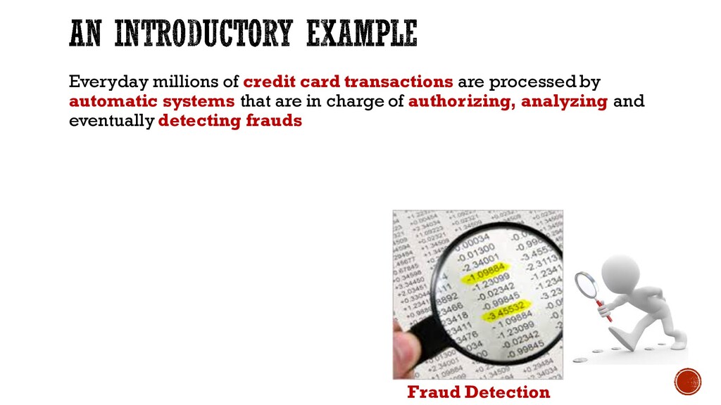
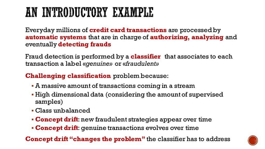
systems that are in charge of authorizing, analyzing and eventually detecting frauds Fraud detection is performed by a classifier that associates to each transaction a label «genuine» or «fraudulent» Challenging classification problem because: § A massive amount of transactions coming in a stream § High dimensional data (considering the amount of supervised samples) § Class unbalanced § Concept drift: new fraudulent strategies appear over time § Concept drift: genuine transactions evolves over time Concept drift “changes the problem” the classifier has to address
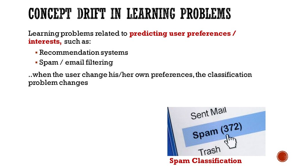
as: § Recommendation systems § Spam / email filtering ..when the user change his/her own preferences, the classification problem changes Spam Classification
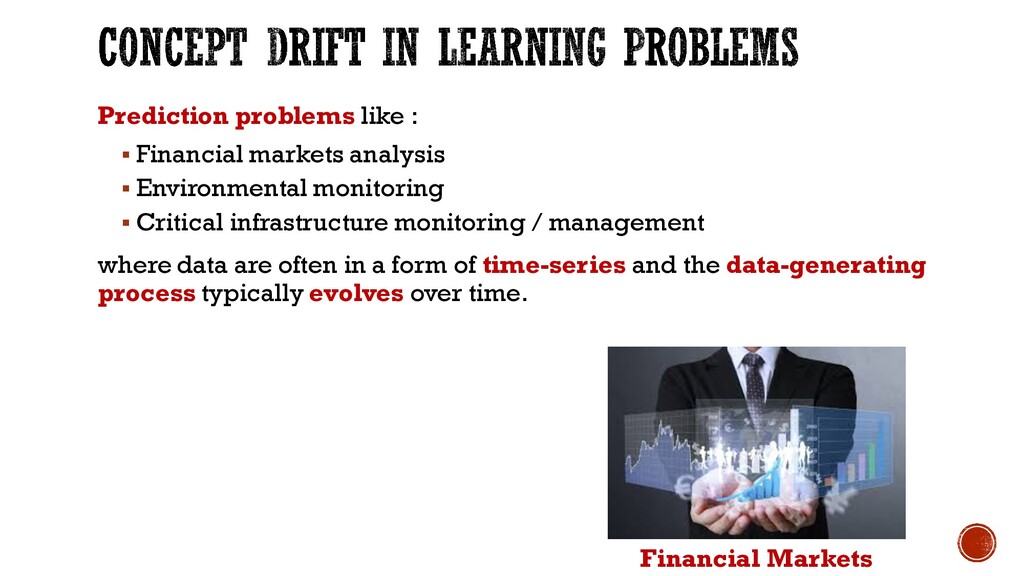
monitoring § Critical infrastructure monitoring / management where data are often in a form of time-series and the data-generating process typically evolves over time. Financial Markets
application scenarios where: § data come in the form of stream § the data-generating process might evolve over time § data-driven models are used Since in these cases, the data-driven model should autonomously adapt to preserve its performance over time
adapting data-driven models to Concept Drift (i.e. in Nonstationary Environments) § learning aspects, while related issues like change/outlier/anomaly detection are not discussed in detail § classification as an example of supervised learning problem. Regression problems are not considered here even though similar issues applies § the most important frameworks that can be implemented using any classifier,rather than solutions for specific classifiers § illustrations typically refer to scalar and numerical data, even though methodologies often apply to multivariate and numerical or categorical data as well
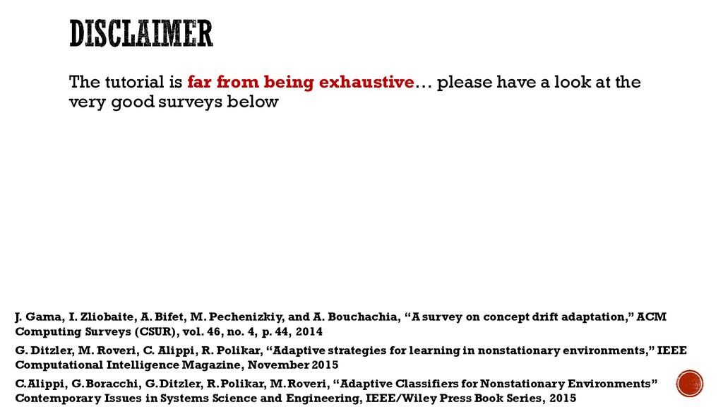
look at the very good surveys below J. Gama, I. Zliobaite, A. Bifet, M. Pechenizkiy, and A. Bouchachia, “A survey on concept drift adaptation,” ACM Computing Surveys (CSUR), vol. 46, no. 4, p. 44, 2014 G. Ditzler, M. Roveri, C. Alippi, R. Polikar, “Adaptive strategies for learning in nonstationary environments,” IEEE Computational Intelligence Magazine, November 2015 C.Alippi, G.Boracchi, G.Ditzler, R.Polikar, M.Roveri, “Adaptive Classifiers for Nonstationary Environments” Contemporary Issues in Systems Science and Engineering, IEEE/Wiley Press Book Series, 2015
look at the very good surveys below We hope this tutorial will help researcher from other disciplines to familiarize with the problem and possibly contribute to the development of this research filed Let’s try to make this tutorial as interactive as possible
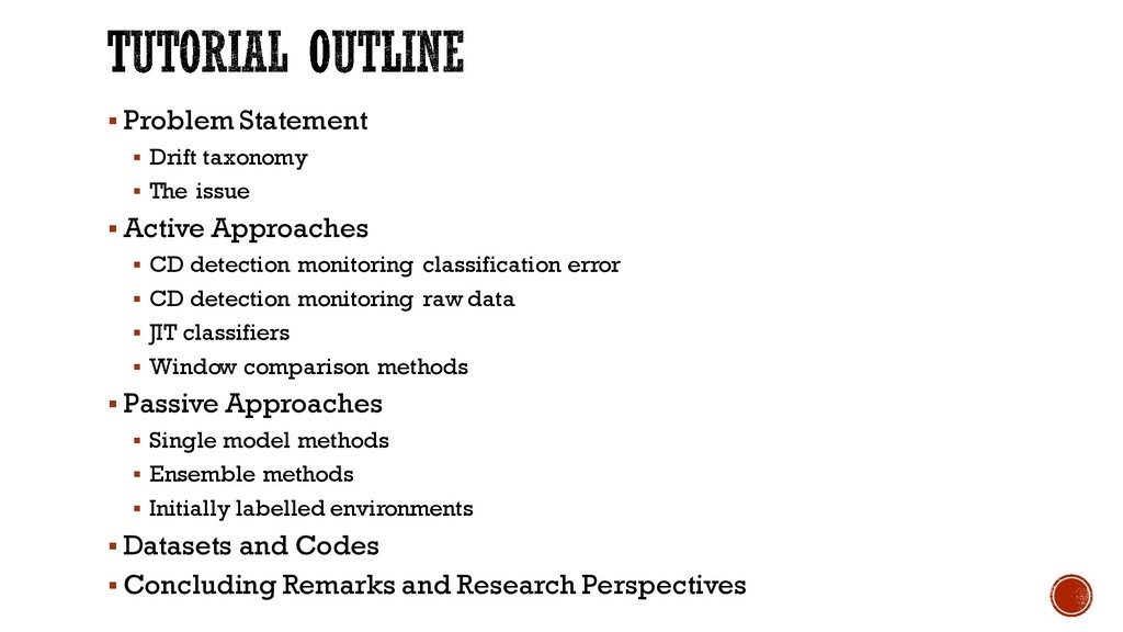
Active Approaches § CD detection monitoring classification error § CD detection monitoring raw data § JIT classifiers § Window comparison methods § Passive Approaches § Single model methods § Ensemble methods § Initially labelled environments § Datasets and Codes § Concluding Remarks and Research Perspectives
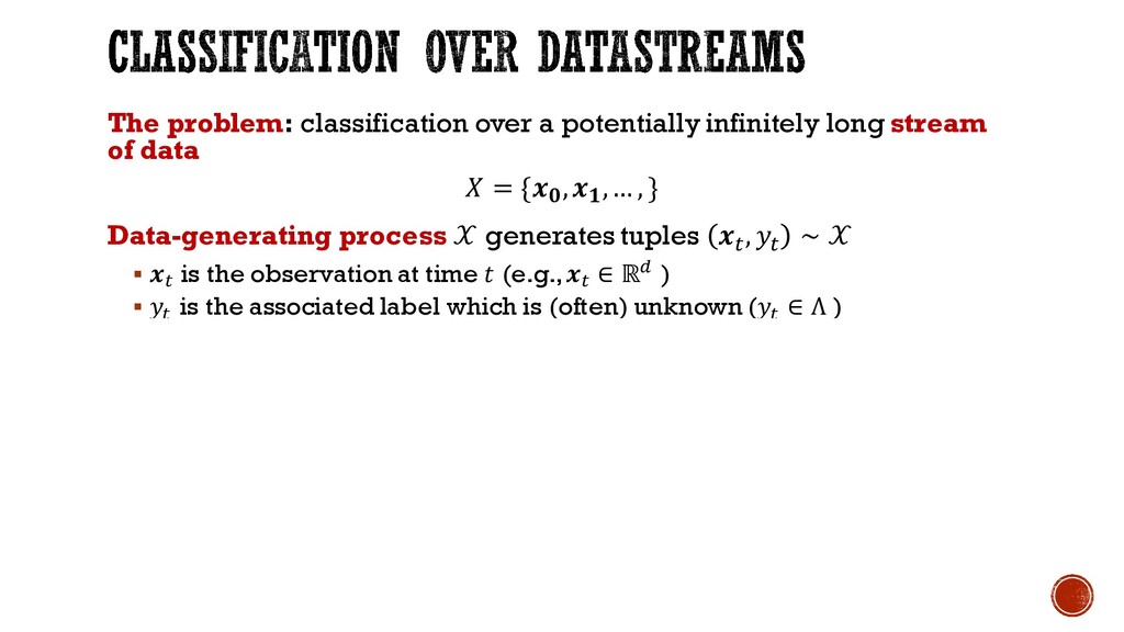
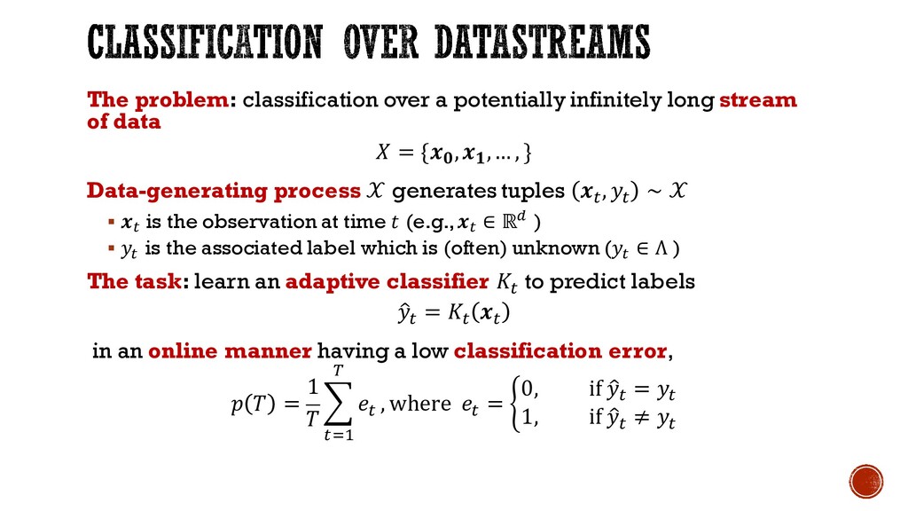
data = { , ,… , } Data-generating process generates tuples + , + ∼ § + is the observation at time (e.g., + ∈ ℝ1 ) § + is the associated label which is (often) unknown (+ ∈ Λ ) The task: learn an adaptive classifier + to predict labels 4+ = + + in an online manner having a low classification error, = 1 8 + : +;< , where + = B 0, if 4+ = + 1, if 4+ ≠ +
data = { , ,… , } Data-generating process generates tuples + , + ∼ § + is the observation at time (e.g., + ∈ ℝ1 ) § + is the associated label which is (often) unknown (+ ∈ Λ ) The task: learn an adaptive classifier + to predict labels 4+ = + + in an online manner having a low classification error, = 1 8 + : +;< , where + = B 0, if 4+ = + 1, if 4+ ≠ +
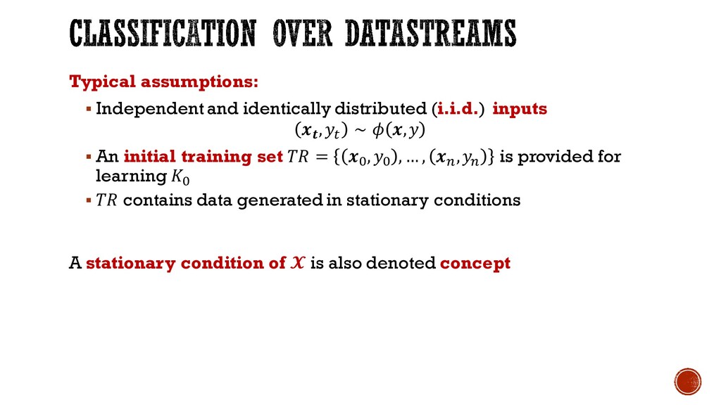
∼ , § An initial training set = J , J , … , K ,K is provided for learning J § contains data generated in stationary conditions A stationary condition of is also denoted concept
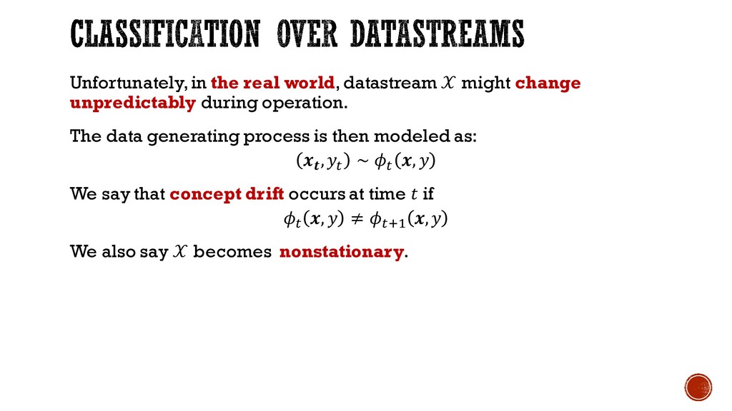
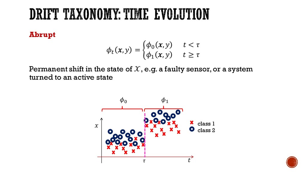
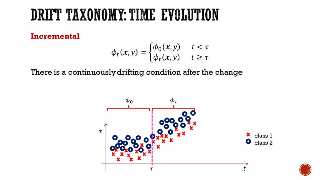
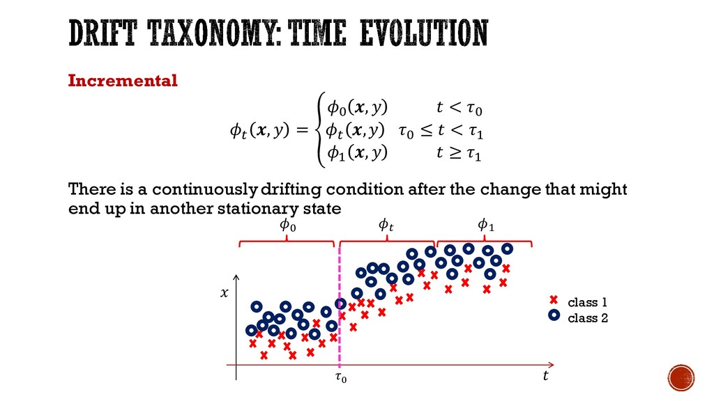
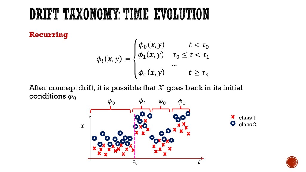
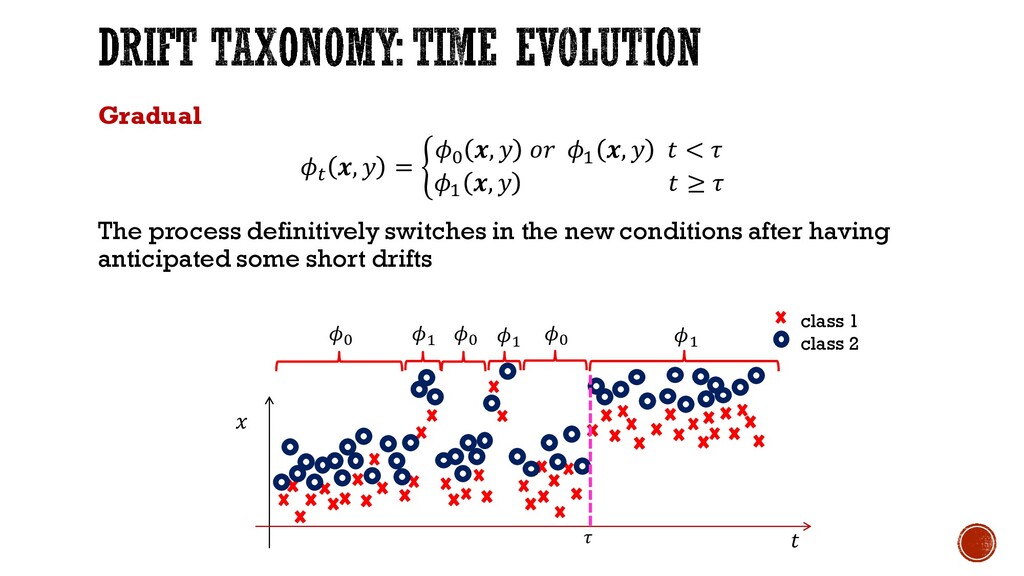
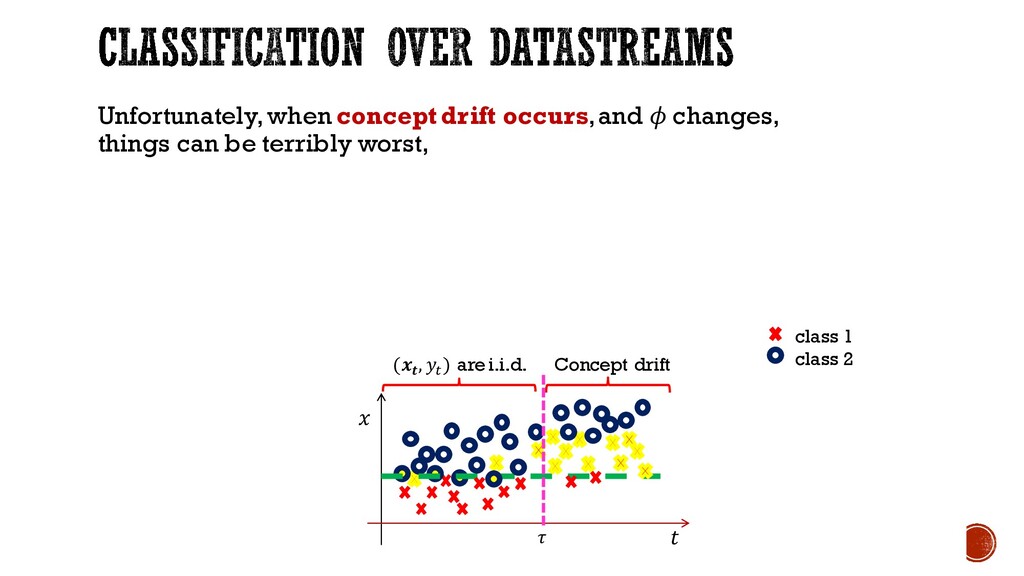
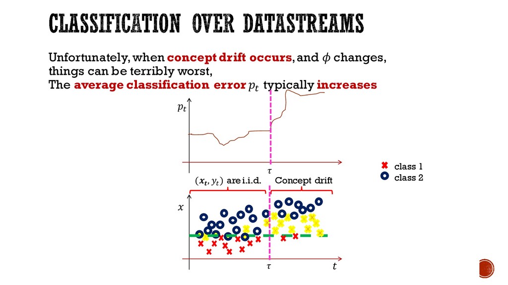
operation. The data generating process is then modeled as: ,+ ∼ + , We say that concept drift occurs at time if + , ≠ +M< , We also say becomes nonstationary.
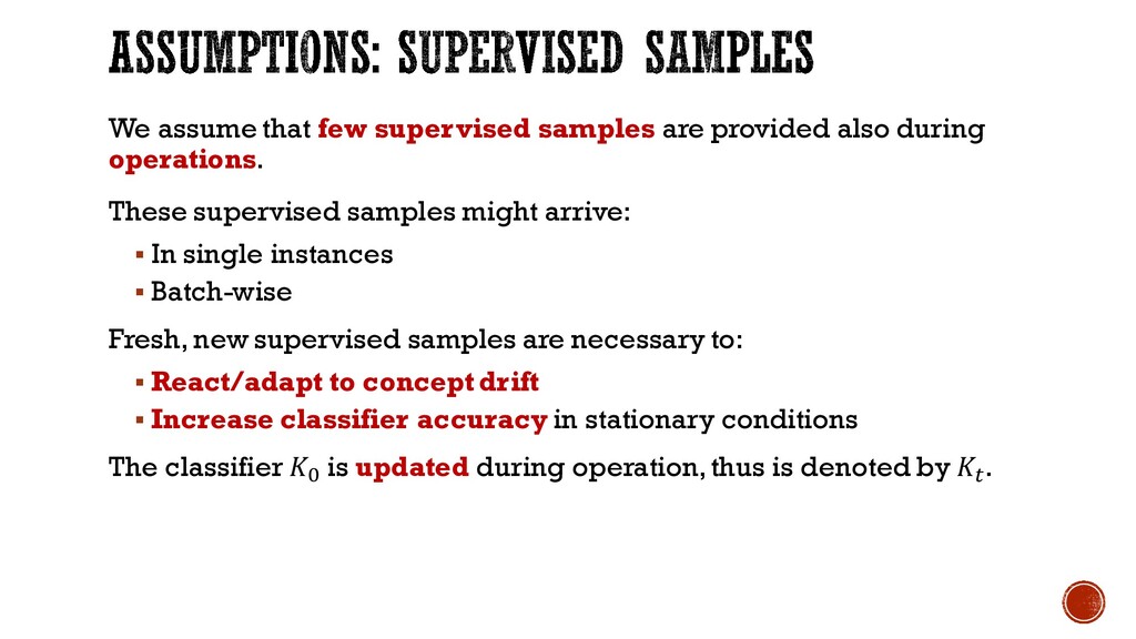
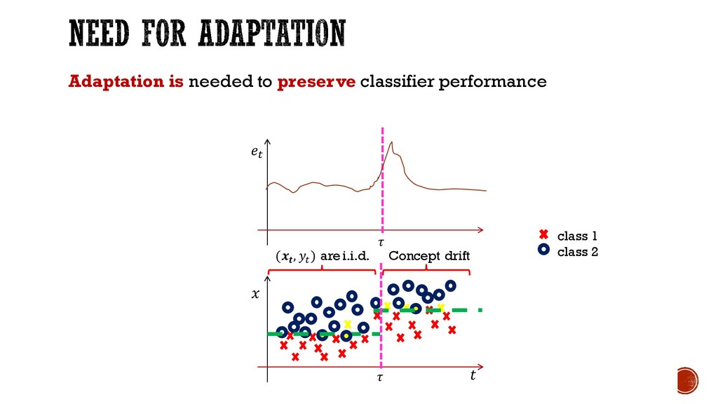
operations. These supervised samples might arrive: § In single instances § Batch-wise Fresh, new supervised samples are necessary to: § React/adapt to concept drift § Increase classifier accuracy in stationary conditions The classifier J is updated during operation, thus is denoted by + .
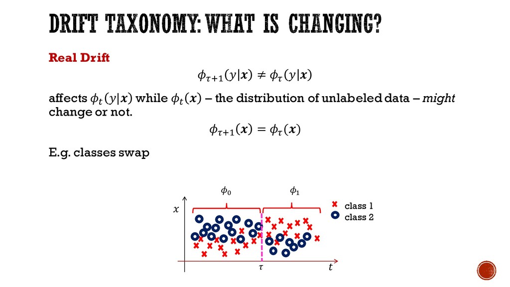
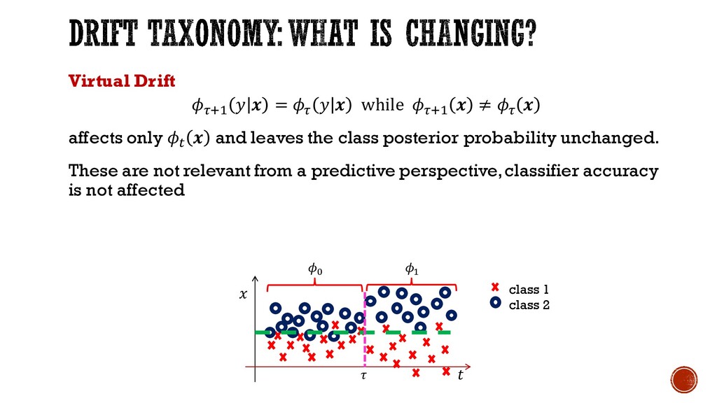
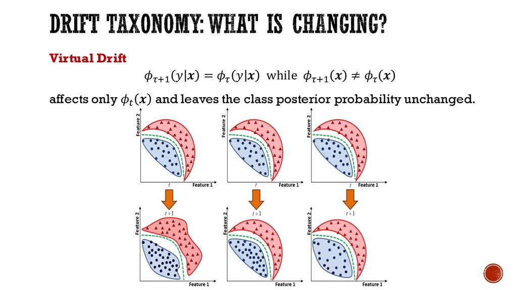
only + and leaves the class posterior probability unchanged. These are not relevant from a predictive perspective, classifier accuracy is not affected class 1 class 2 J <
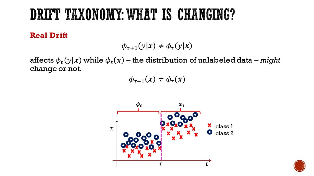
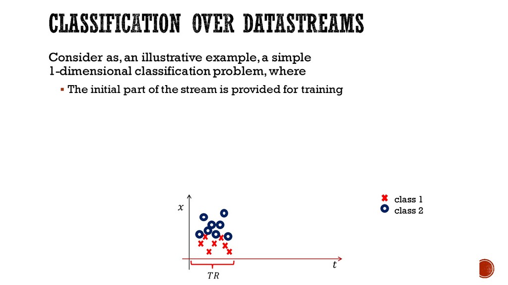
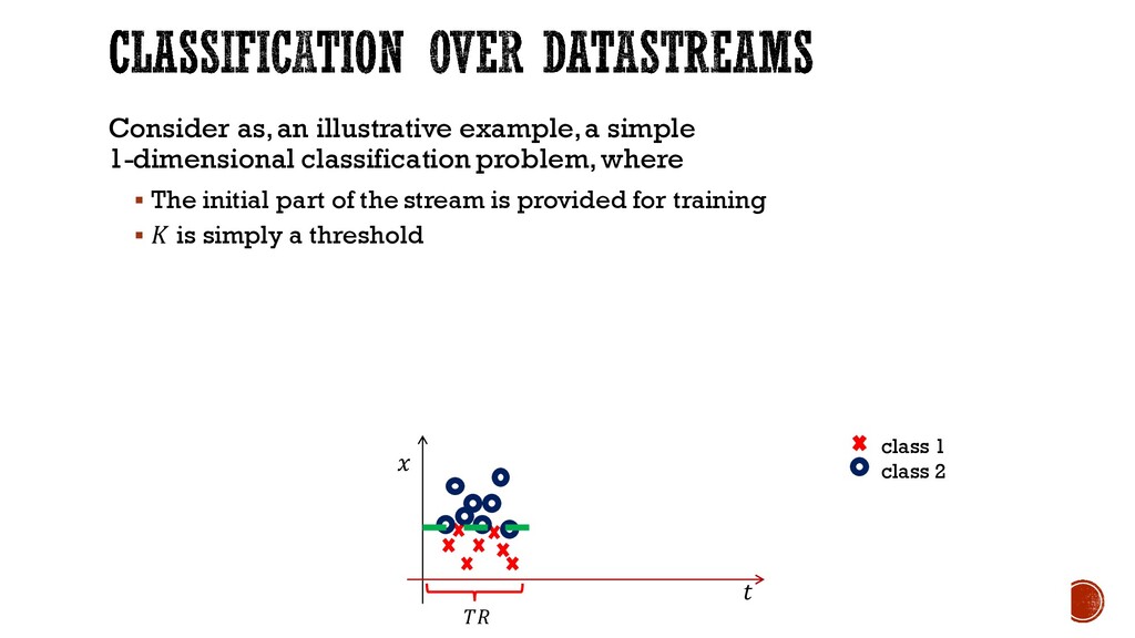
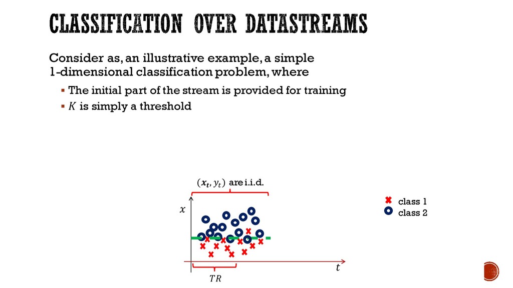
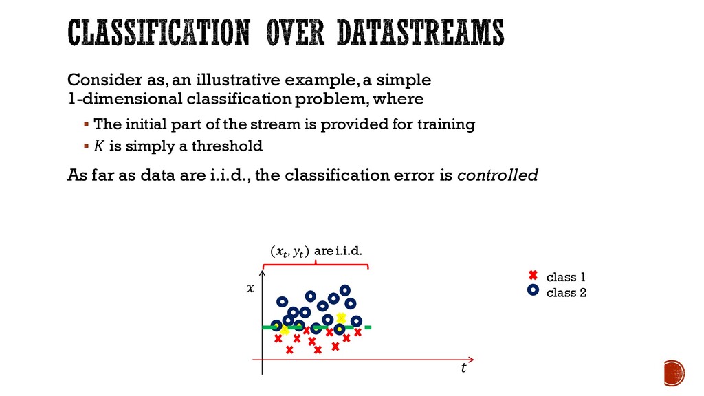
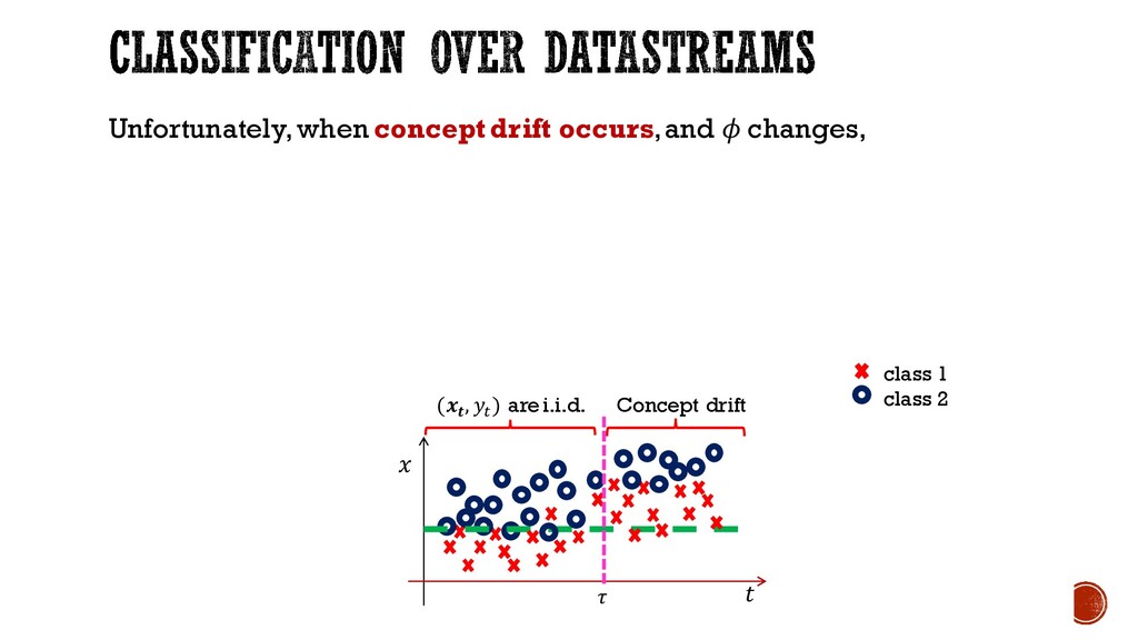
where § The initial part of the stream is provided for training § is simply a threshold As far as data are i.i.d., the classification error is controlled ( , + ) are i.i.d. class 1 class 2
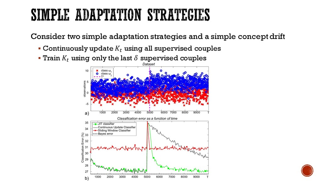
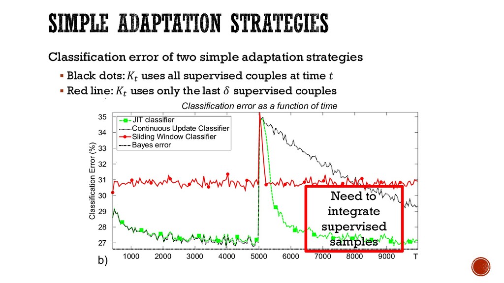
§ Continuously update + using all supervised couples § Train + using only the last supervised couples observations -5 0 5 10 class ω class ω T* Classification error as a function of time Classification Error (%) 1000 2000 3000 4000 5000 6000 7000 8000 9000 27 28 29 30 31 32 33 34 35 T JIT classifier Continuous Update Classifier Sliding Window Classifier Bayes error Dataset 1 2 a) b) 1000 2000 3000 4000 5000 6000 7000 8000 9000 T
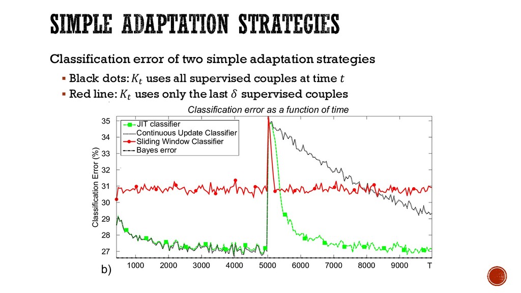
+ uses all supervised couples at time § Red line: + uses only the last supervised couples observations -5 0 5 T* Classification error as a function of time Classification Error (%) 1000 2000 3000 4000 5000 6000 7000 8000 9000 27 28 29 30 31 32 33 34 35 T JIT classifier Continuous Update Classifier Sliding Window Classifier Bayes error a) b) 1000 2000 3000 4000 5000 6000 7000 8000 9000 T
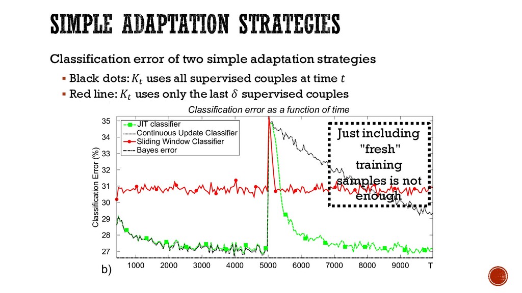
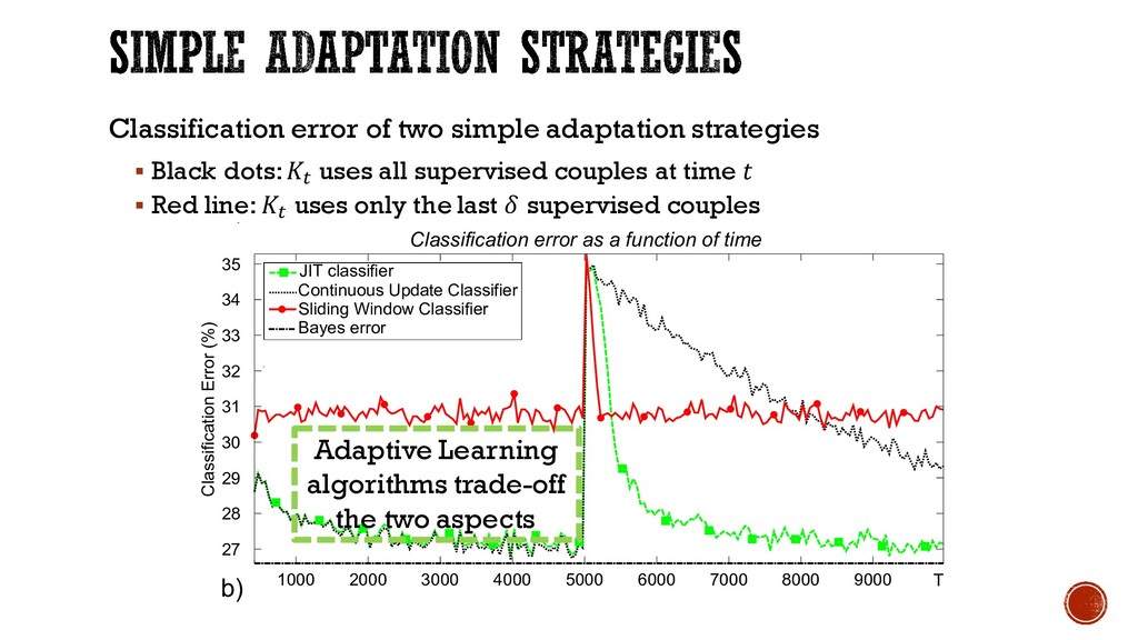
+ uses all supervised couples at time § Red line: + uses only the last supervised couples observations -5 0 5 T* Classification error as a function of time Classification Error (%) 1000 2000 3000 4000 5000 6000 7000 8000 9000 27 28 29 30 31 32 33 34 35 T JIT classifier Continuous Update Classifier Sliding Window Classifier Bayes error a) b) 1000 2000 3000 4000 5000 6000 7000 8000 9000 T Just including "fresh" training samples is not enough
+ uses all supervised couples at time § Red line: + uses only the last supervised couples observations -5 0 5 T* Classification error as a function of time Classification Error (%) 1000 2000 3000 4000 5000 6000 7000 8000 9000 27 28 29 30 31 32 33 34 35 T JIT classifier Continuous Update Classifier Sliding Window Classifier Bayes error a) b) 1000 2000 3000 4000 5000 6000 7000 8000 9000 T Need to integrate supervised samples
+ uses all supervised couples at time § Red line: + uses only the last supervised couples observations -5 0 5 T* Classification error as a function of time Classification Error (%) 1000 2000 3000 4000 5000 6000 7000 8000 9000 27 28 29 30 31 32 33 34 35 T JIT classifier Continuous Update Classifier Sliding Window Classifier Bayes error a) b) 1000 2000 3000 4000 5000 6000 7000 8000 9000 T Adaptive Learning algorithms trade-off the two aspects
+ is combined with statistical tools to detect concept drift and pilot the adaptation § Passive: the classifier + undergoes continuous adaptation determining every time which supervised information to preserve Which is best depends on the expected change rate and memory/computational availability
Elettronica e Informazione Milano, Italy 2 The University of Arizona Department of Electrical & Computer Engineering Tucson, AZ USA [email protected], [email protected]
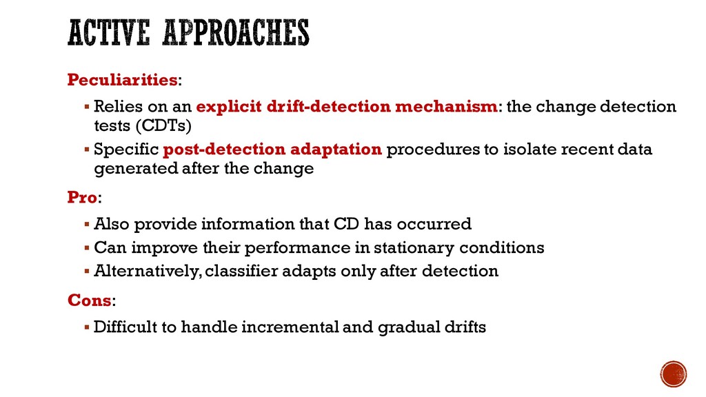
detection tests (CDTs) § Specific post-detection adaptation procedures to isolate recent data generated after the change Pro: § Also provide information that CD has occurred § Can improve their performance in stationary conditions § Alternatively, classifier adapts only after detection Cons: § Difficult to handle incremental and gradual drifts
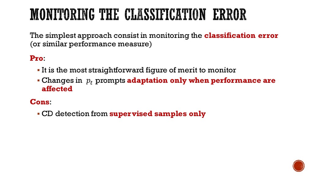
similar performance measure) Pro: § It is the most straightforward figure of merit to monitor § Changes in + prompts adaptation only when performance are affected Cons: § CD detection from supervised samples only
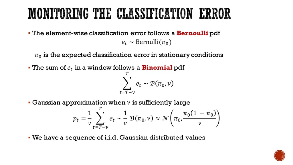
∼ Bernulli(J ) J is the expected classification error in stationary conditions § The sum of + in a window follows a Binomial pdf 8 + : +;:`a ∼ ℬ J , § Gaussian approximation when is sufficiently large + = 1 8 + : +;:`a ∼ 1 ℬ J , ≈ J , J 1 − J § We have a sequence of i.i.d. Gaussian distributed values
Medas, G. Castillo, and P. Rodrigues. “Learning with Drift Detection” In Proc. of the 17th Brazilian Symp. on Artif. Intell. (SBIA). Springer, Berlin, 286–295, 2004
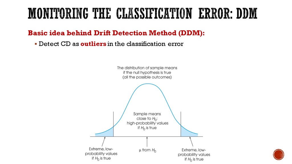
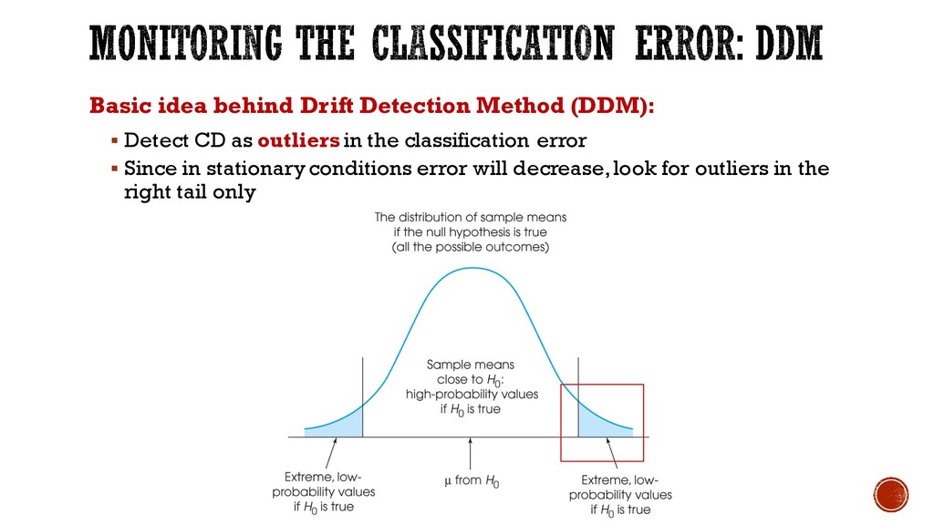
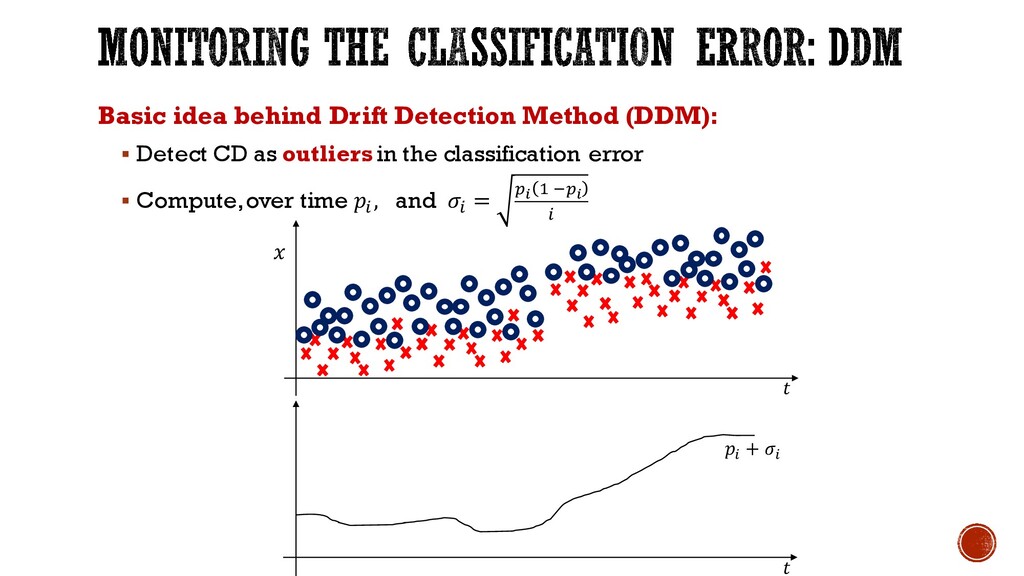
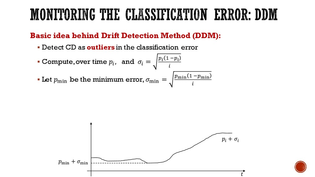
as outliers in the classification error § Compute, over time g , and g = ij < `ij g § Let lmn be the minimum error, lmn = iopq < `iopq g g + g lmn + lmn
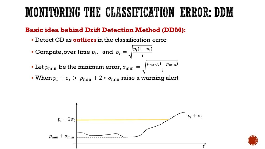
as outliers in the classification error § Compute, over time g , and g = ij < `ij g § Let lmn be the minimum error, lmn = iopq < `iopq g § When g + g > lmn + 2 ∗ lmn raise a warning alert g + g lmn + lmn g + 2g
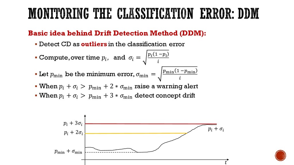
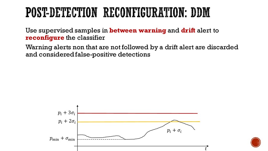
as outliers in the classification error § Compute, over time g , and g = ij < `ij g § Let lmn be the minimum error, lmn = iopq < `iopq g § When g + g > lmn + 2 ∗ lmn raise a warning alert § When g + g > lmn + 3 ∗ lmn detect concept drift g + g lmn + lmn g + 3g g + 2g
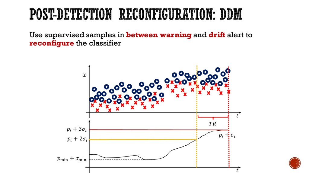
reconfigure the classifier Warning alerts non that are not followed by a drift alert are discarded and considered false-positive detections lmn + lmn g + 3g g + 2g g + g
average distance between misclassified samples § Average distance is expected to decrease under CD § They aim at detecting gradual drifts M. Baena-García, J. Campo-Ávila, R. Fidalgo, A. Bifet, R. Gavaldá, R. Morales-Bueno. “Early drift detection method“ In Fourth International Workshop on Knowledge Discovery from Data Streams (2006)
Compute EWMA statistic + = 1 − +`< + + , J = 0 Detect concept drift when + > J,+ + + + § J,+ is the average error estimated until time § + is its standard deviation of the above estimator § + is a threshold parameter EWMA statistic is mainly influenced by recent data. CD is detected when the error on recent samples departs from J,+ G. J. Ross, N. M. Adams, D. K. Tasoulis, and D. J. Hand "Exponentially Weighted Moving Average Charts for Detecting Concept Drift" Pattern Recogn. Lett. 33, 2 (Jan. 2012), 191–198 2012
average run length (ARL) of the test (the expected time between false positives) § Like DDM, classifier reconfiguration is performed by monitoring + also at a warning level + > J,+ + 0.5 + + § Once CD is detected, the first sample raising a warning is used to isolate samples from the new distribution and retrain the classifier G. J. Ross, N. M. Adams, D. K. Tasoulis, and D. J. Hand "Exponentially Weighted Moving Average Charts for Detecting Concept Drift" Pattern Recogn. Lett. 33, 2 (Jan. 2012), 191–198 2012
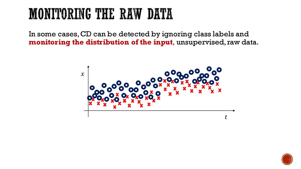
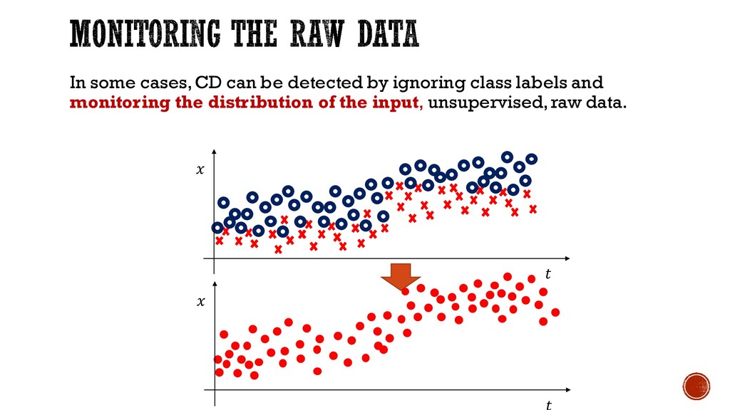
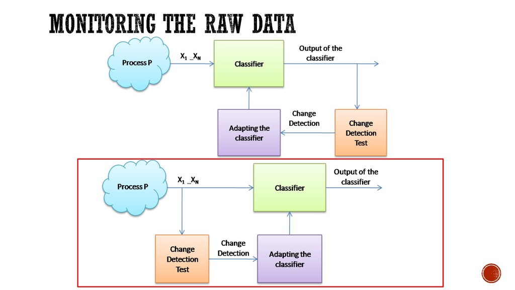
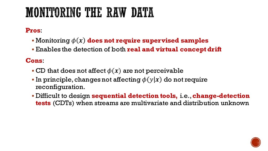
the detection of both real and virtual concept drift Cons: § CD that does not affect () are not perceivable § In principle, changes not affecting do not require reconfiguration. § Difficult to design sequential detection tools, i.e., change-detection tests (CDTs) when streams are multivariate and distribution unknown
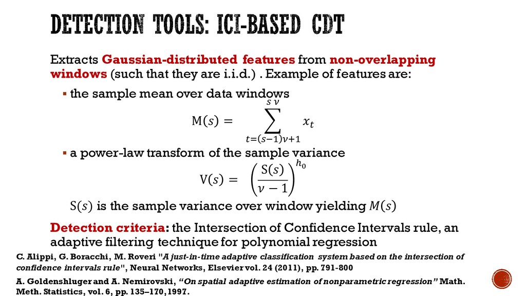
i.i.d.) . Example of features are: § the sample mean over data windows M = 8 + } a +; }`< aM< § a power-law transform of the sample variance V = S − 1 €• S() is the sample variance over window yielding Detection criteria: the Intersection of Confidence Intervals rule, an adaptive filtering technique for polynomial regression C. Alippi, G. Boracchi, M. Roveri "A just-in-time adaptive classification system based on the intersection of confidence intervals rule", Neural Networks, Elsevier vol. 24 (2011), pp. 791-800 A. Goldenshluger and A. Nemirovski, “On spatial adaptive estimation of nonparametric regression” Math. Meth. Statistics, vol. 6, pp. 135–170,1997.
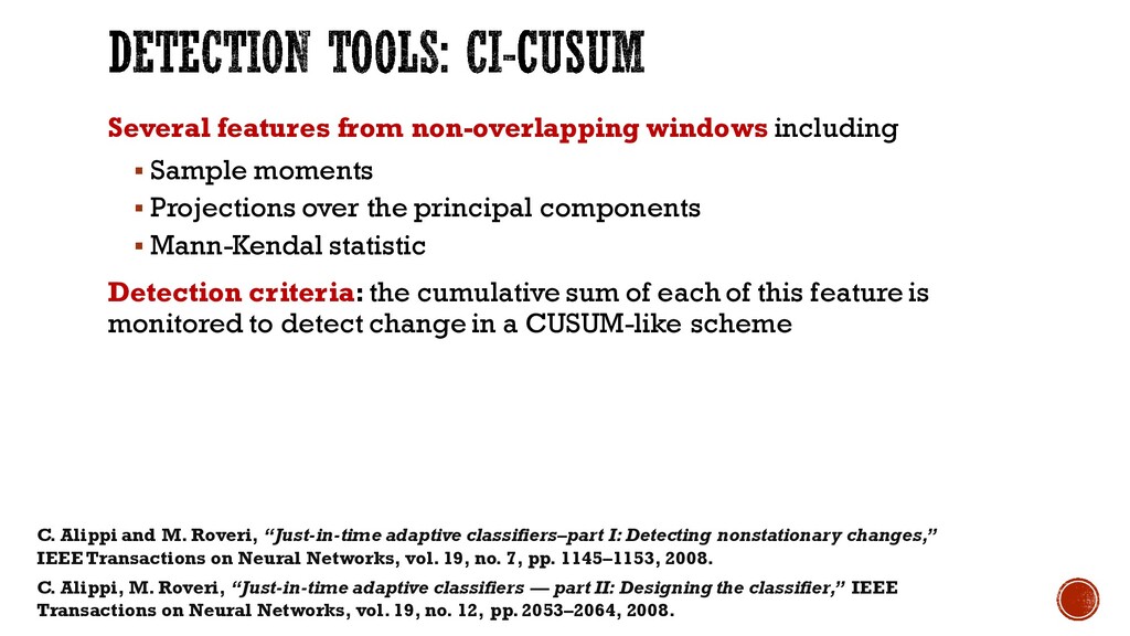
Projections over the principal components § Mann-Kendal statistic Detection criteria: the cumulative sum of each of this feature is monitored to detect change in a CUSUM-like scheme C. Alippi and M. Roveri, “Just-in-time adaptive classifiers–part I: Detecting nonstationary changes,” IEEE Transactions on Neural Networks, vol. 19, no. 7, pp. 1145–1153, 2008. C. Alippi, M. Roveri, “Just-in-time adaptive classifiers — part II: Designing the classifier,” IEEE Transactions on Neural Networks, vol. 19, no. 12, pp. 2053–2064, 2008.
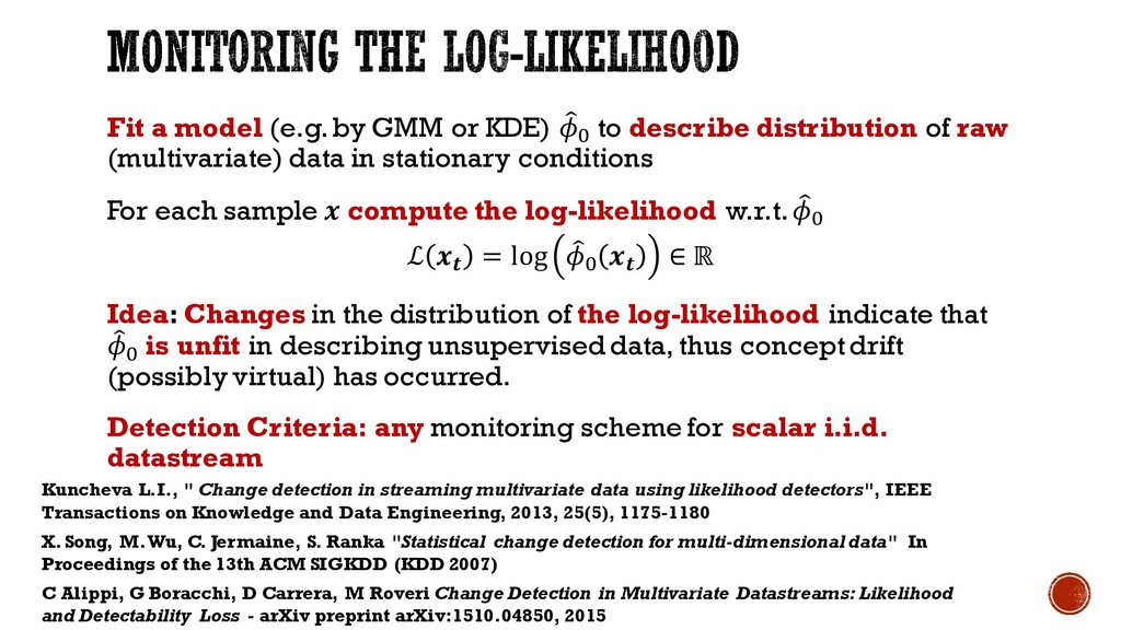
to describe distribution of raw (multivariate) data in stationary conditions For each sample compute the log-likelihood w.r.t. ƒ J ℒ = log ƒ J ∈ ℝ Idea: Changes in the distribution of the log-likelihood indicate that ƒ J is unfit in describing unsupervised data, thus concept drift (possibly virtual) has occurred. Detection Criteria: any monitoring scheme for scalar i.i.d. datastream Kuncheva L.I., " Change detection in streaming multivariate data using likelihood detectors", IEEE Transactions on Knowledge and Data Engineering, 2013, 25(5), 1175-1180 X. Song, M. Wu, C. Jermaine, S. Ranka "Statistical change detection for multi-dimensional data" In Proceedings of the 13th ACM SIGKDD (KDD 2007) C Alippi, G Boracchi, D Carrera, M Roveri Change Detection in Multivariate Datastreams: Likelihood and Detectability Loss - arXiv preprint arXiv:1510.04850, 2015
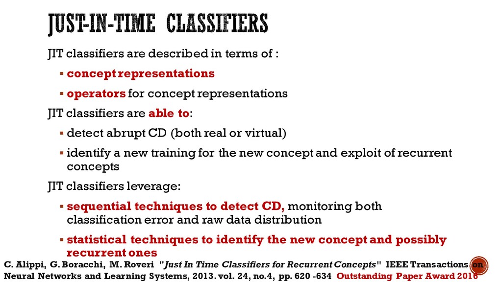
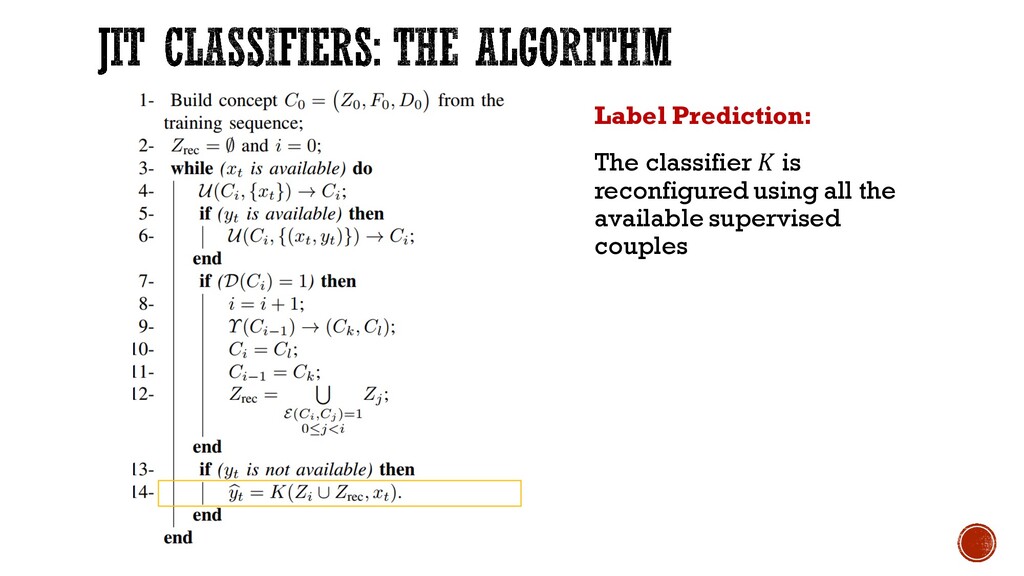
representations § operators for concept representations JIT classifiers are able to: § detect abrupt CD (both real or virtual) § identify a new training for the new concept and exploit of recurrent concepts JIT classifiers leverage: § sequential techniques to detect CD, monitoring both classification error and raw data distribution § statistical techniques to identify the new concept and possibly recurrent ones C. Alippi, G. Boracchi, M. Roveri "Just In Time Classifiers for Recurrent Concepts" IEEE Transactions on Neural Networks and Learning Systems, 2013. vol. 24, no.4, pp. 620 -634 Outstanding Paper Award 2016
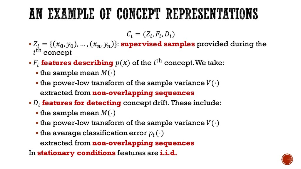
= ,J , … , ,K : supervised samples provided during the •Ž concept § g features describing () of the •Ž concept. We take: § the sample mean ⋅ § the power-low transform of the sample variance (⋅) extracted from non-overlapping sequences § g features for detecting concept drift. These include: § the sample mean ⋅ § the power-low transform of the sample variance (⋅) § the average classification error + (⋅) extracted from non-overlapping sequences In stationary conditions features are i.i.d.
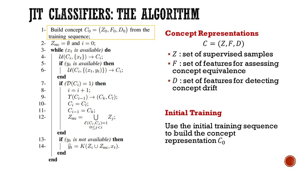
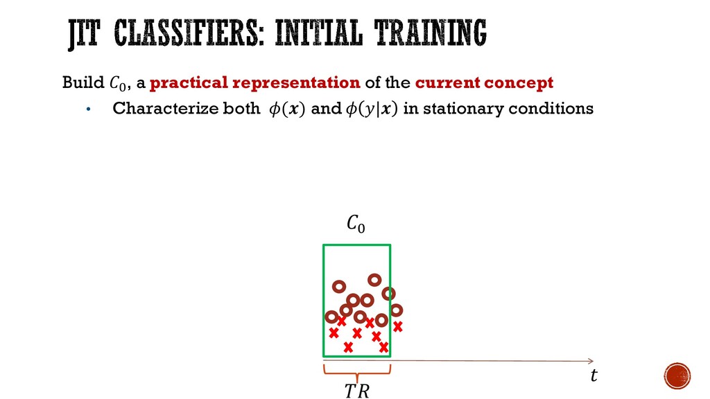
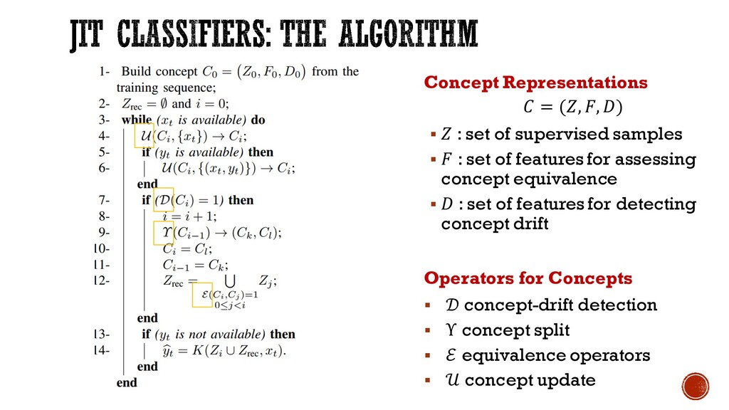
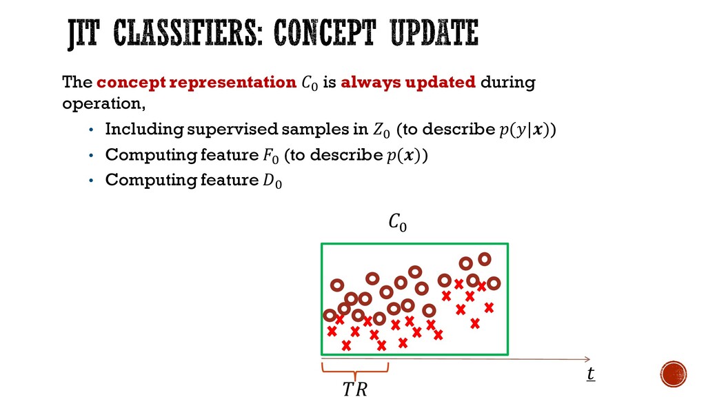
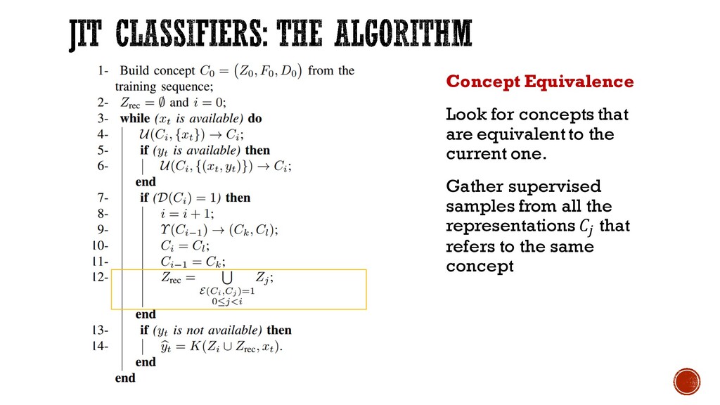
samples § : set of features for assessing concept equivalence § : set of features for detecting concept drift Initial Training Use the initial training sequence to build the concept representation J
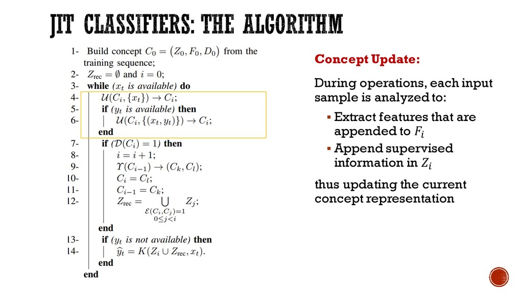
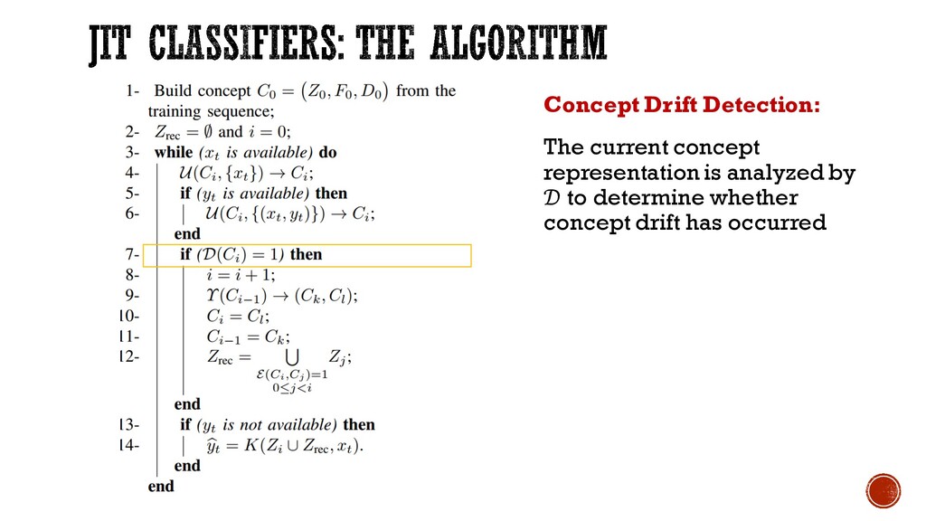
supervised samples § : set of features for assessing concept equivalence § : set of features for detecting concept drift Operators for Concepts § concept-drift detection § Υ concept split § ℰ equivalence operators § concept update
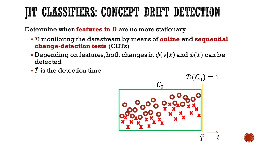
the datastream by means of online and sequential change-detection tests (CDTs) § Depending on features, both changes in and () can be detected § ƒ is the detection time ƒ J (J ) = 1
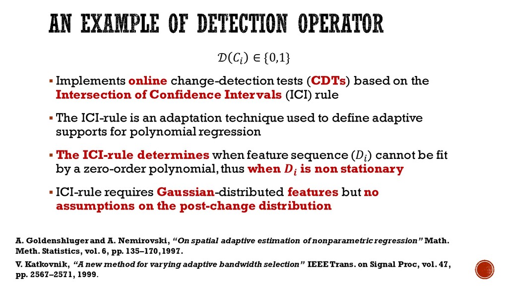
on the Intersection of Confidence Intervals (ICI) rule § The ICI-rule is an adaptation technique used to define adaptive supports for polynomial regression § The ICI-rule determines when feature sequence (g ) cannot be fit by a zero-order polynomial, thus when is non stationary § ICI-rule requires Gaussian-distributed features but no assumptions on the post-change distribution A. Goldenshluger and A. Nemirovski, “On spatial adaptive estimation of nonparametric regression” Math. Meth. Statistics, vol. 6, pp. 135–170,1997. V. Katkovnik, “A new method for varying adaptive bandwidth selection” IEEE Trans. on Signal Proc, vol. 47, pp. 2567–2571, 1999.
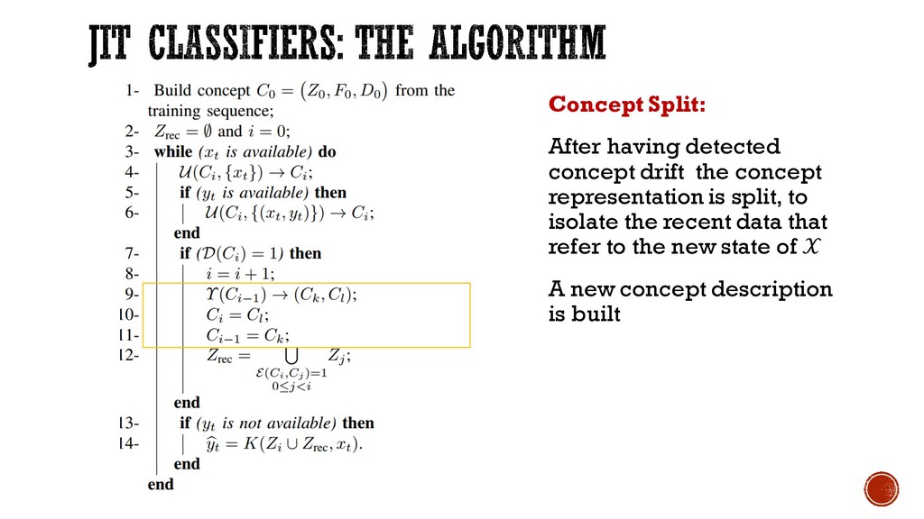
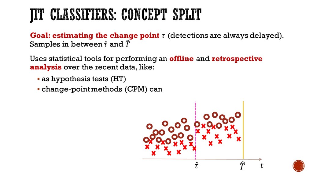
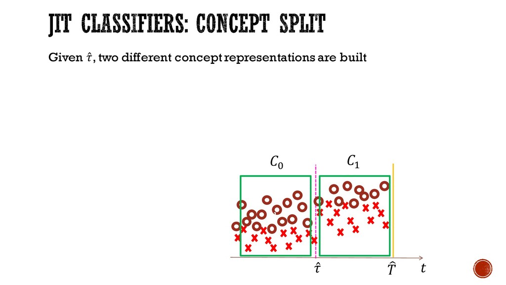
in between ̂ and ƒ Uses statistical tools for performing an offline and retrospective analysis over the recent data, like: § as hypothesis tests (HT) § change-point methods (CPM) can ƒ ̂
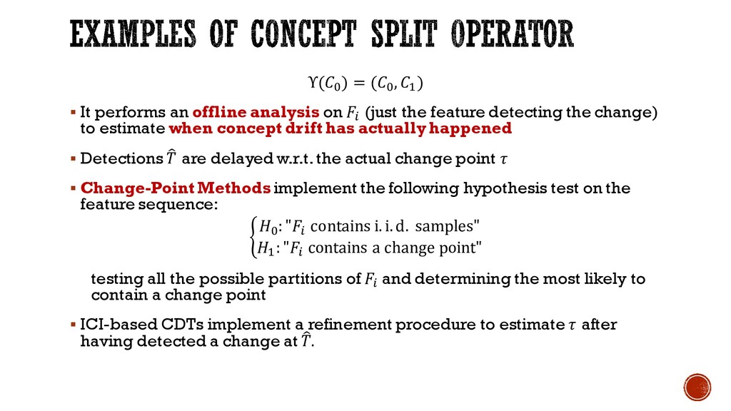
an offline analysis on g (just the feature detecting the change) to estimate when concept drift has actually happened § Detections ƒ are delayed w.r.t. the actual change point § Change-Point Methods implement the following hypothesis test on the feature sequence: B J :"g contains i. i. d. samples" < :"g contains a change point" testing all the possible partitions of g and determining the most likely to contain a change point § ICI-based CDTs implement a refinement procedure to estimate after having detected a change at ƒ.
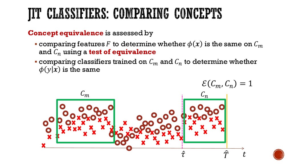
whether is the same on ¢ and K using a test of equivalence § comparing classifiers trained on ¢ and K to determine whether is the same ƒ K ¢ ℰ ¢ , K = 1 ̂
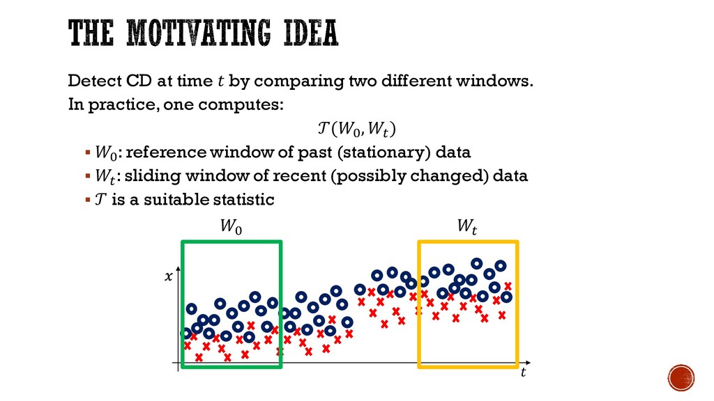
practice, one computes: (J , + ) § J : reference window of past (stationary) data § + : sliding window of recent (possibly changed) data § is a suitable statistic J +
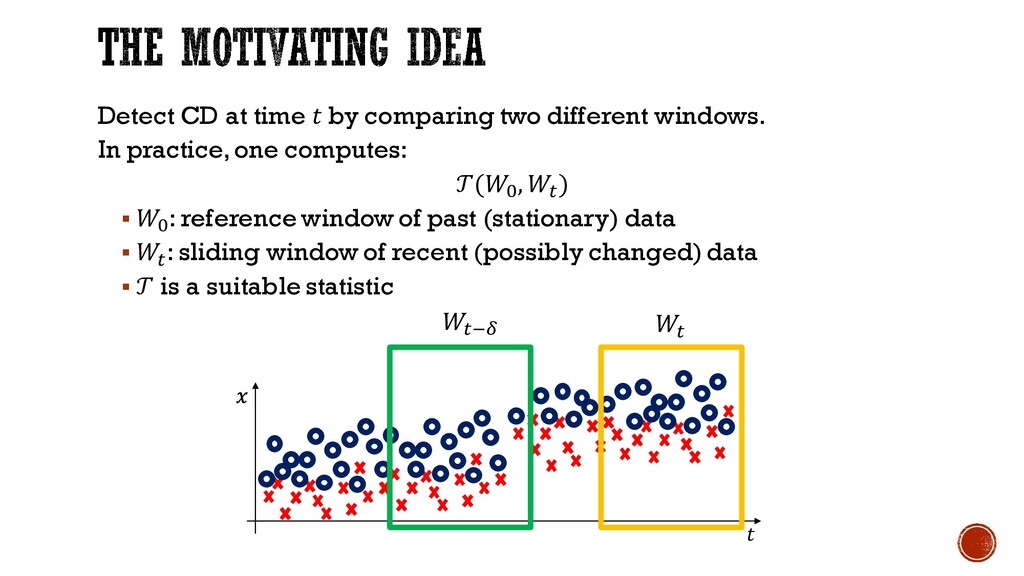
practice, one computes: (J , + ) § J : reference window of past (stationary) data § + : sliding window of recent (possibly changed) data § is a suitable statistic +`¥ +
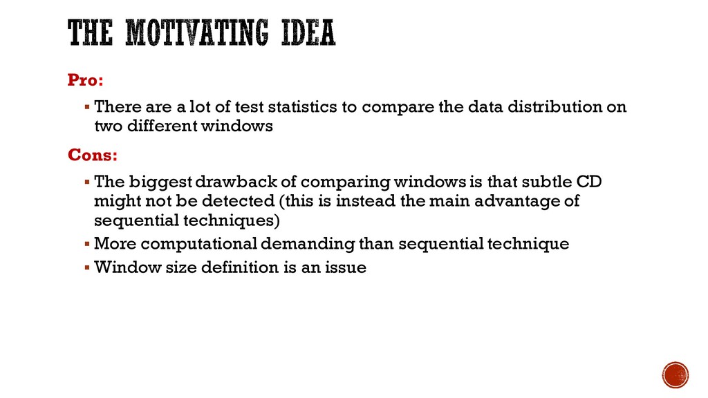
compare the data distribution on two different windows Cons: § The biggest drawback of comparing windows is that subtle CD might not be detected (this is instead the main advantage of sequential techniques) § More computational demanding than sequential technique § Window size definition is an issue
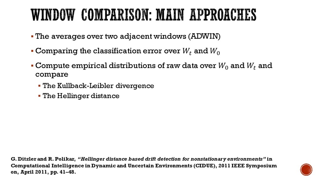
the classification error over + and J § Compute empirical distributions of raw data over J and + and compare § The Kullback-Leibler divergence T. Dasu, Sh. Krishnan, S. Venkatasubramanian, and K. Yi. "An Information-Theoretic Approach to Detecting Changes in Multi-Dimensional Data Streams". In Proc. of the 38th Symp. on the Interface of Statistics, Computing Science, and Applications, 2006
the classification error over + and J § Compute empirical distributions of raw data over J and + and compare § The Kullback-Leibler divergence § The Hellinger distance G. Ditzler and R. Polikar, “Hellinger distance based drift detection for nonstationary environments” in Computational Intelligence in Dynamic and Uncertain Environments (CIDUE), 2011 IEEE Symposium on, April 2011, pp. 41–48.
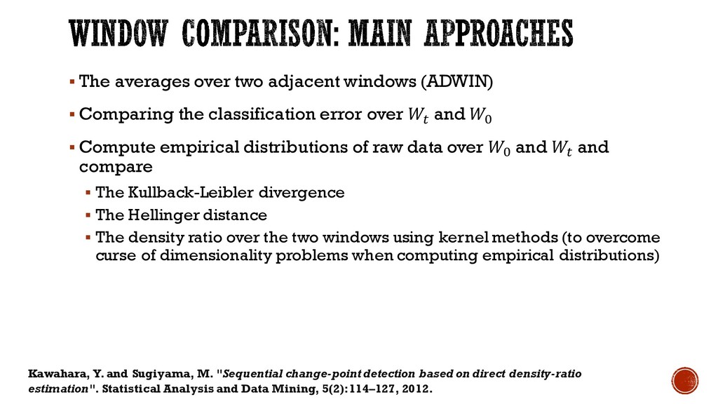
the classification error over + and J § Compute empirical distributions of raw data over J and + and compare § The Kullback-Leibler divergence § The Hellinger distance § The density ratio over the two windows using kernel methods (to overcome curse of dimensionality problems when computing empirical distributions) Kawahara, Y. and Sugiyama, M. "Sequential change-point detection based on direct density-ratio estimation". Statistical Analysis and Data Mining, 5(2):114–127, 2012.
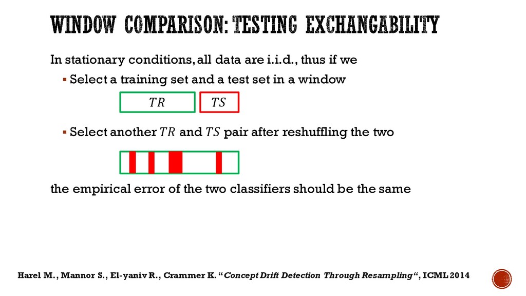
§ Select a training set and a test set in a window § Select another and pair after reshuffling the two the empirical error of the two classifiers should be the same Harel M., Mannor S., El-yaniv R., Crammer K. “Concept Drift Detection Through Resampling“, ICML 2014
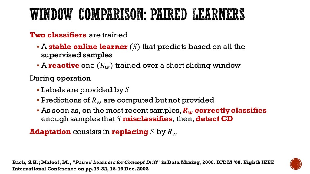
that predicts based on all the supervised samples § A reactive one (§ ) trained over a short sliding window During operation § Labels are provided by § Predictions of § are computed but not provided § As soon as, on the most recent samples, correctly classifies enough samples that misclassifies, then, detect CD Adaptation consists in replacing by § Bach, S.H.; Maloof, M., "Paired Learners for Concept Drift" in Data Mining, 2008. ICDM '08. Eighth IEEE International Conference on pp.23-32, 15-19 Dec. 2008
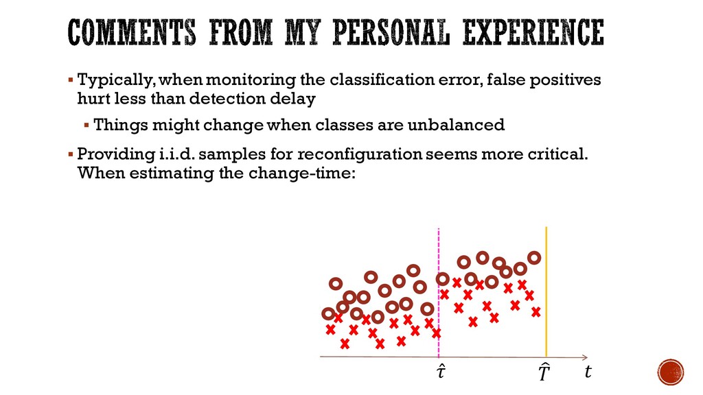
less than detection delay § Things might change when classes are unbalanced § Providing i.i.d. samples for reconfiguration seems more critical. When estimating the change-time: ƒ ̂
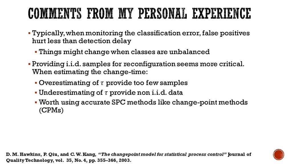
less than detection delay § Things might change when classes are unbalanced § Providing i.i.d. samples for reconfiguration seems more critical. When estimating the change-time: § Overestimating of provide too few samples § Underestimating of provide non i.i.d. data § Worth using accurate SPC methods like change-point methods (CPMs) D. M. Hawkins, P. Qiu, and C. W. Kang, “The changepoint model for statistical process control” Journal of Quality Technology, vol. 35, No. 4, pp. 355–366, 2003.
less than detection delay § Things might change when classes are unbalanced § Providing i.i.d. samples for reconfiguration seems more critical. When estimating the change-time: § Overestimating of provide too few samples § Underestimating of provide non i.i.d. data § Worth using accurate SPC methods like change-point methods (CPMs) § Exploiting recurrent concepts is important § Providing additional samples could really make the difference § Mitigate the impact of false positives