Chapters 3 & 4. Many of the topics discussed today fall under the umbrella of unsupervised learning. That is learning from unlabeled data. Topics Parametric: maximum likelihood estimator, Bayesian estimation Non–parametric: kernel density estimation, mixture models, generalized view of EM Clustering: k–means, expectation maximization About the figures: many of the figures were collected from the Pattern Classification & PRML text, along with some figures generated by custom Matlab and Python scripts. Also, much of the content of the lecture is derived from previous years lectures of this course. Gregory Ditzler Pattern Recognition & Machine Learning
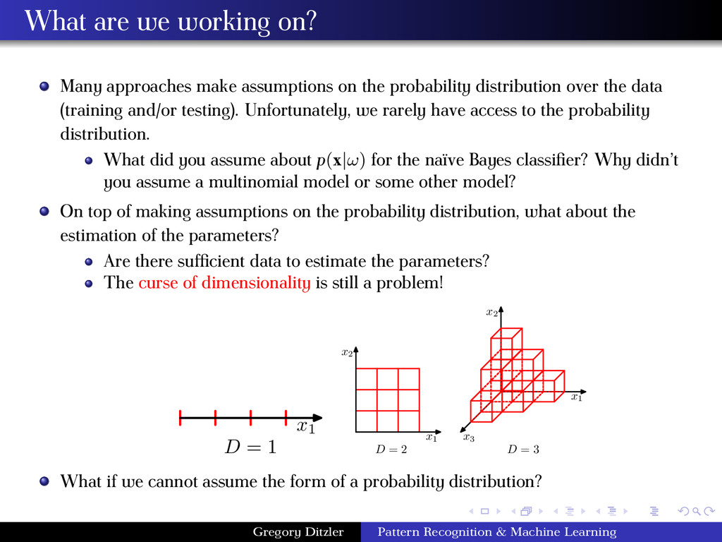
the probability distribution over the data (training and/or testing). Unfortunately, we rarely have access to the probability distribution. What did you assume about p(x|ω) for the naïve Bayes classifier? Why didn’t you assume a multinomial model or some other model? On top of making assumptions on the probability distribution, what about the estimation of the parameters? Are there sufficient data to estimate the parameters? The curse of dimensionality is still a problem! x1 D = 1 x1 x2 D = 2 x1 x2 x3 D = 3 What if we cannot assume the form of a probability distribution? Gregory Ditzler Pattern Recognition & Machine Learning
the properties and computation of functions such as p(x) that govern the behavior of a probability distribution. For example, if X is distributed as a Gaussian random variable, then the probability distribution for X has parameters µ and σ2. The distribution is of the form, p(X = x) = 1 √ 2πσ e− (x−µ)2 2σ2 The Bayes classifier required that you know P(ω), p(x|ω), and p(x) p(x) can be computed using the total probability theorem What if the distribution on ω and/or the x’s conditional distribution on ω is unknown? We can assume the form of the distribution, but how do we know if it is correct or approximately correct? One option is to use the Kolmorogrov-Smirnov test to test against a distribution How much data are sufficient to estimate the parameters? If we can (cannot) assume the form of the distribution, we use parametric (nonparametric) techniques Gregory Ditzler Pattern Recognition & Machine Learning
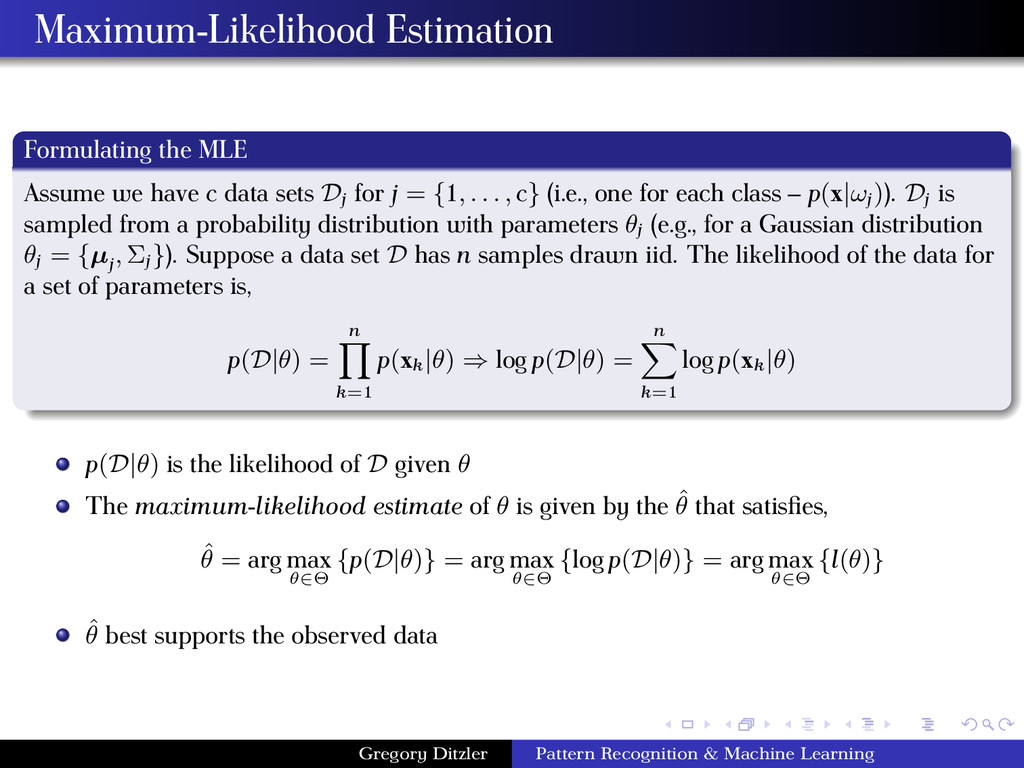
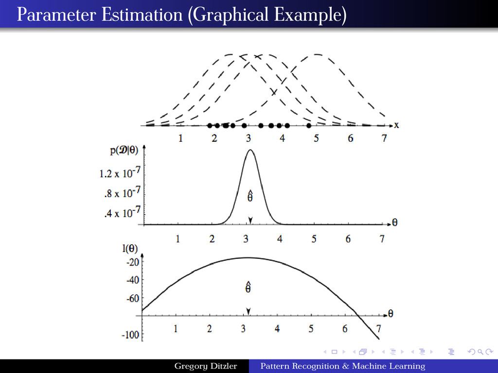
sets Dj for j = {1, . . . , c} (i.e., one for each class – p(x|ωj )). Dj is sampled from a probability distribution with parameters θj (e.g., for a Gaussian distribution θj = {µj , Σj }). Suppose a data set D has n samples drawn iid. The likelihood of the data for a set of parameters is, p(D|θ) = n k=1 p(xk |θ) ⇒ log p(D|θ) = n k=1 log p(xk |θ) p(D|θ) is the likelihood of D given θ The maximum-likelihood estimate of θ is given by the ˆ θ that satisfies, ˆ θ = arg max θ∈Θ {p(D|θ)} = arg max θ∈Θ {log p(D|θ)} = arg max θ∈Θ {l(θ)} ˆ θ best supports the observed data Gregory Ditzler Pattern Recognition & Machine Learning
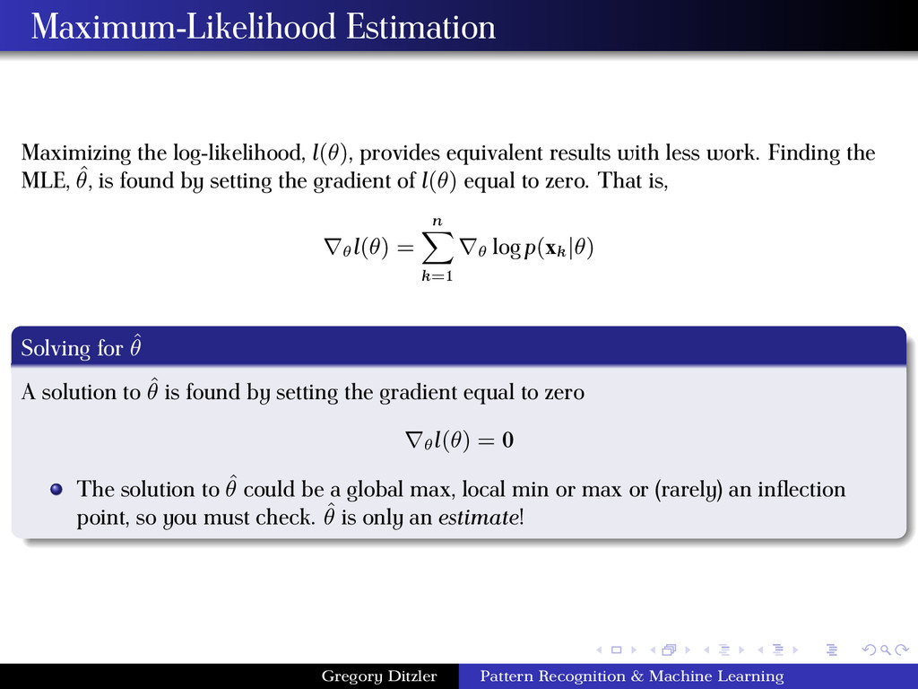
less work. Finding the MLE, ˆ θ, is found by setting the gradient of l(θ) equal to zero. That is, ∇θ l(θ) = n k=1 ∇θ log p(xk |θ) Solving for ˆ θ A solution to ˆ θ is found by setting the gradient equal to zero ∇θ l(θ) = 0 The solution to ˆ θ could be a global max, local min or max or (rarely) an inflection point, so you must check. ˆ θ is only an estimate! Gregory Ditzler Pattern Recognition & Machine Learning
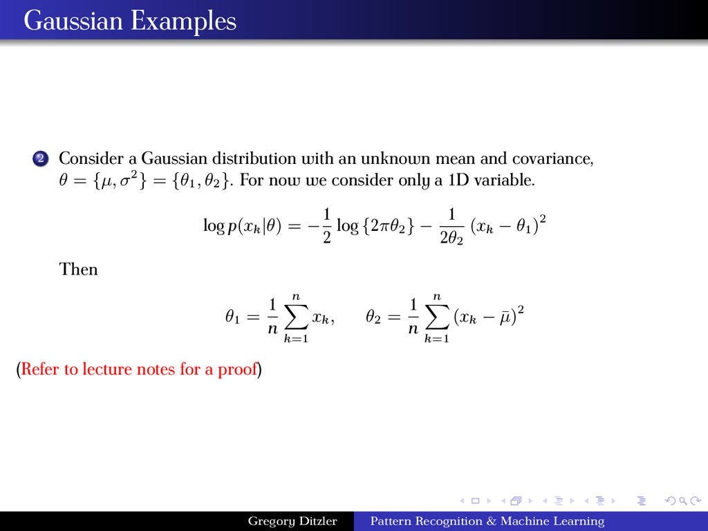
mean and covariance, θ = {µ, σ2} = {θ1 , θ2 }. For now we consider only a 1D variable. log p(xk |θ) = − 1 2 log {2πθ2 } − 1 2θ2 (xk − θ1 )2 Then θ1 = 1 n n k=1 xk , θ2 = 1 n n k=1 (xk − ¯ µ)2 (Refer to lecture notes for a proof) Gregory Ditzler Pattern Recognition & Machine Learning
are these estimates? We assess the goodness and reliability through Bias: How close is the estimate to the true value? E[ˆ θ] = θ? Variance: How much would this estimate change, had we tried this again with a different dataset also drawn from the same distribution? Gregory Ditzler Pattern Recognition & Machine Learning
biased; however we can make it unbiased by using σ2 ∗ = n n−1 ¯ σ2. The sample mean is an unbiased estimator for µ. As n → ∞, the estimator’s bias is negligible; however, it will always be biased. One of the very important properties of the maximum likelihood estimate is that it is invariant to non-linear transformations Other estimators exist for parameter estimation such as the minimum variance unbiased estimator (MVUE) Gregory Ditzler Pattern Recognition & Machine Learning
to be fixed, but unknown. Bayesian Estimation (BE) assumes θ are random variables and instead of finding ˆ θ we find p(θ|D). BE generally provides us with more information; however, computing θBE may be more involved than θMLE . Bayesian estimation is not estimating θ, rather we are finding the distribution p(x|D) based on the observation of D For most practical applications, if the assumptions are correct, and there is sufficient data MLE gives good results MLE: Frequentist approach BE: Bayesian approach The MLE method found the estimator that maximized the log-likelihood function, p(D|θ). Why didn’t we use the a priori density p(θ|D)? Such methods that use p(θ|D) are referred to as Bayesian estimation techniques. Gregory Ditzler Pattern Recognition & Machine Learning
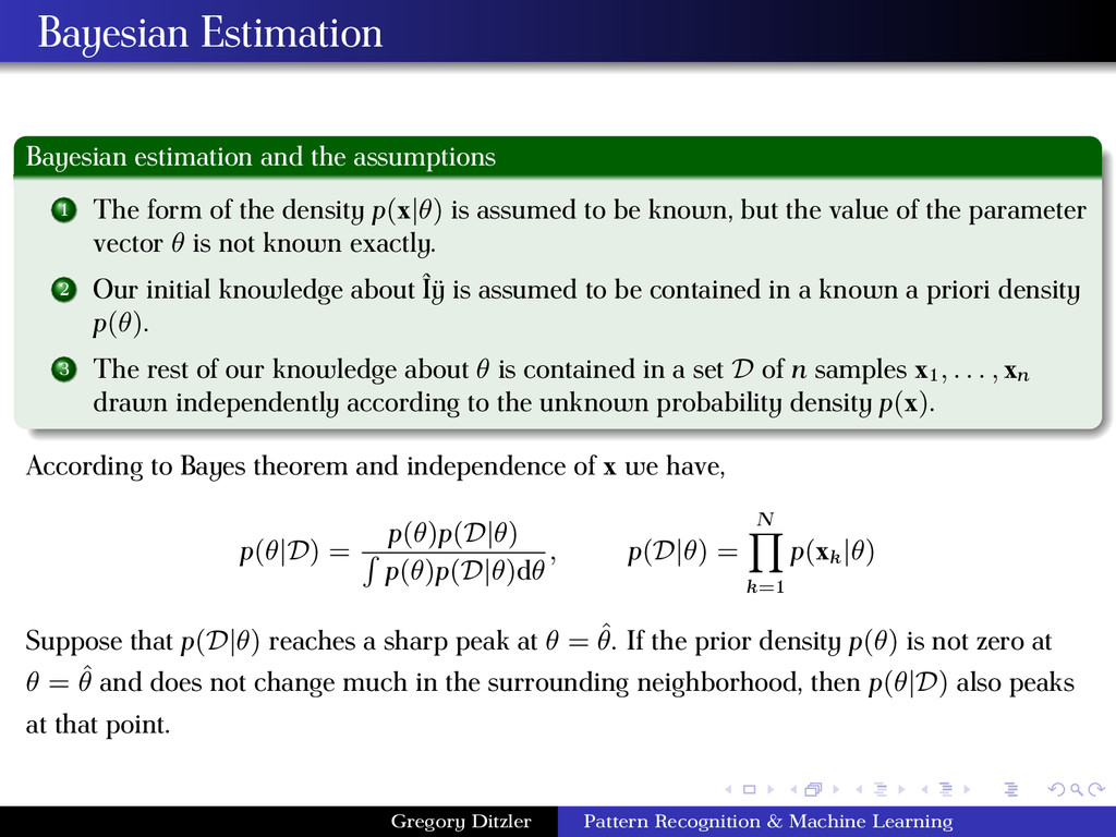
of the density p(x|θ) is assumed to be known, but the value of the parameter vector θ is not known exactly. 2 Our initial knowledge about Îÿ is assumed to be contained in a known a priori density p(θ). 3 The rest of our knowledge about θ is contained in a set D of n samples x1 , . . . , xn drawn independently according to the unknown probability density p(x). According to Bayes theorem and independence of x we have, p(θ|D) = p(θ)p(D|θ) p(θ)p(D|θ)dθ , p(D|θ) = N k=1 p(xk |θ) Suppose that p(D|θ) reaches a sharp peak at θ = ˆ θ. If the prior density p(θ) is not zero at θ = ˆ θ and does not change much in the surrounding neighborhood, then p(θ|D) also peaks at that point. Gregory Ditzler Pattern Recognition & Machine Learning
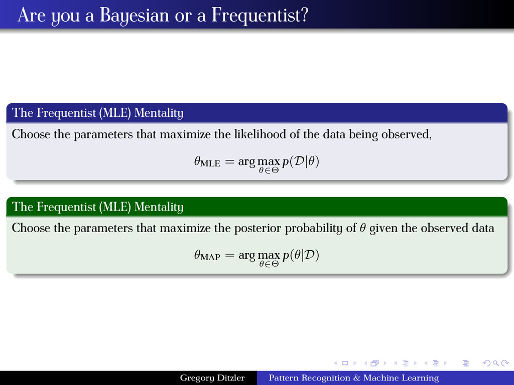
Mentality Choose the parameters that maximize the likelihood of the data being observed, θMLE = arg max θ∈Θ p(D|θ) The Frequentist (MLE) Mentality Choose the parameters that maximize the posterior probability of θ given the observed data θMAP = arg max θ∈Θ p(θ|D) Gregory Ditzler Pattern Recognition & Machine Learning
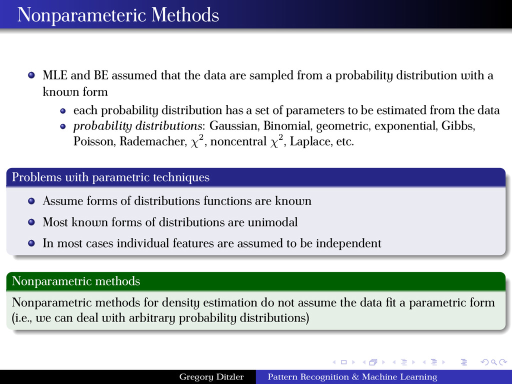
sampled from a probability distribution with a known form each probability distribution has a set of parameters to be estimated from the data probability distributions: Gaussian, Binomial, geometric, exponential, Gibbs, Poisson, Rademacher, χ2, noncentral χ2, Laplace, etc. Problems with parametric techniques Assume forms of distributions functions are known Most known forms of distributions are unimodal In most cases individual features are assumed to be independent Nonparametric methods Nonparametric methods for density estimation do not assume the data fit a parametric form (i.e., we can deal with arbitrary probability distributions) Gregory Ditzler Pattern Recognition & Machine Learning
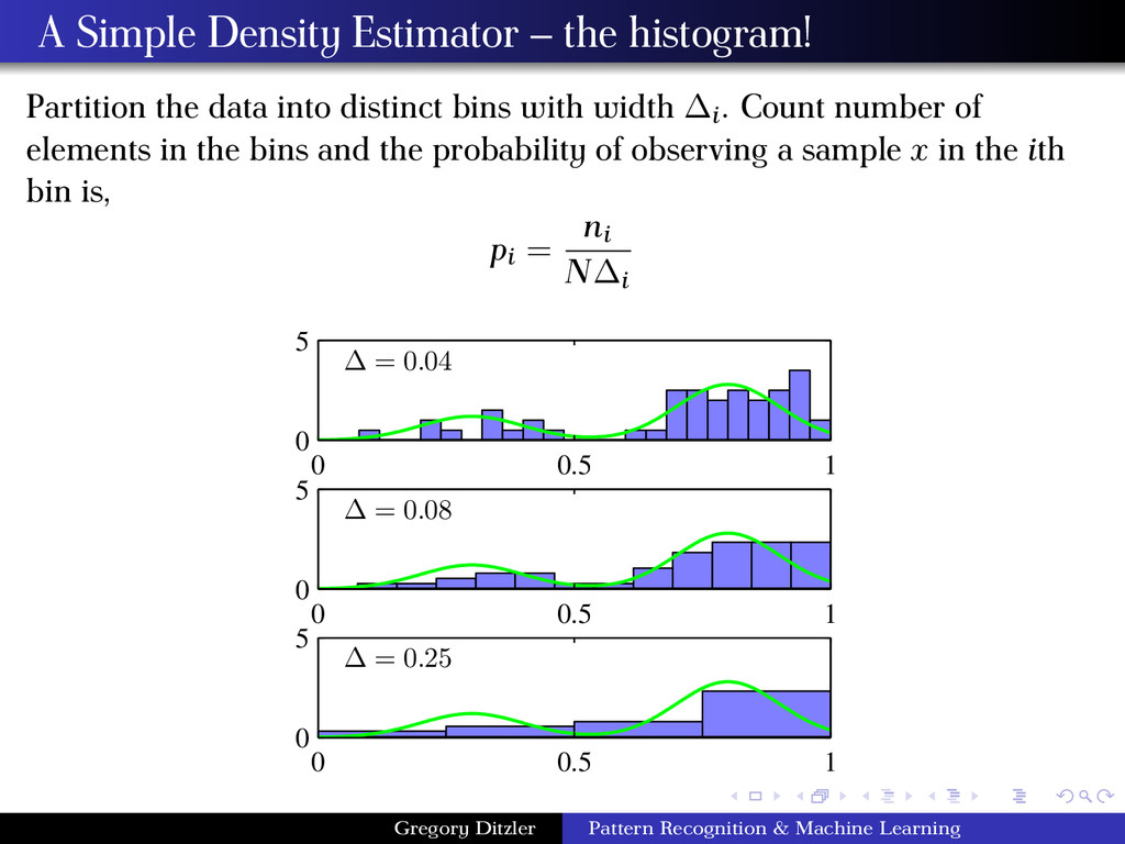
into distinct bins with width ∆i. Count number of elements in the bins and the probability of observing a sample x in the ith bin is, pi = ni N∆i ∆ = 0.04 0 0.5 1 0 5 ∆ = 0.08 0 0.5 1 0 5 ∆ = 0.25 0 0.5 1 0 5 Gregory Ditzler Pattern Recognition & Machine Learning
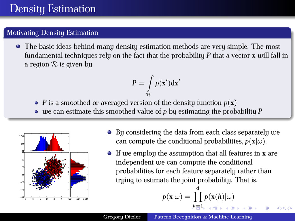
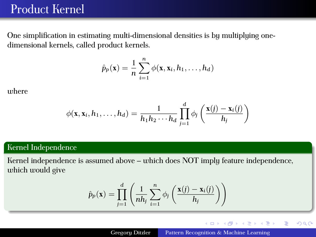
density estimation methods are very simple. The most fundamental techniques rely on the fact that the probability P that a vector x will fall in a region R is given by P = R p(x )dx P is a smoothed or averaged version of the density function p(x) we can estimate this smoothed value of p by estimating the probability P 6 4 2 0 2 4 6 6 4 2 0 2 4 6 0 50 100 0 50 100 By considering the data from each class separately we can compute the conditional probabilities, p(x|ω). If we employ the assumption that all features in x are independent we can compute the conditional probabilities for each feature separately rather than trying to estimate the joint probability. That is, p(x|ω) = d k=1 p(x(k)|ω) Gregory Ditzler Pattern Recognition & Machine Learning
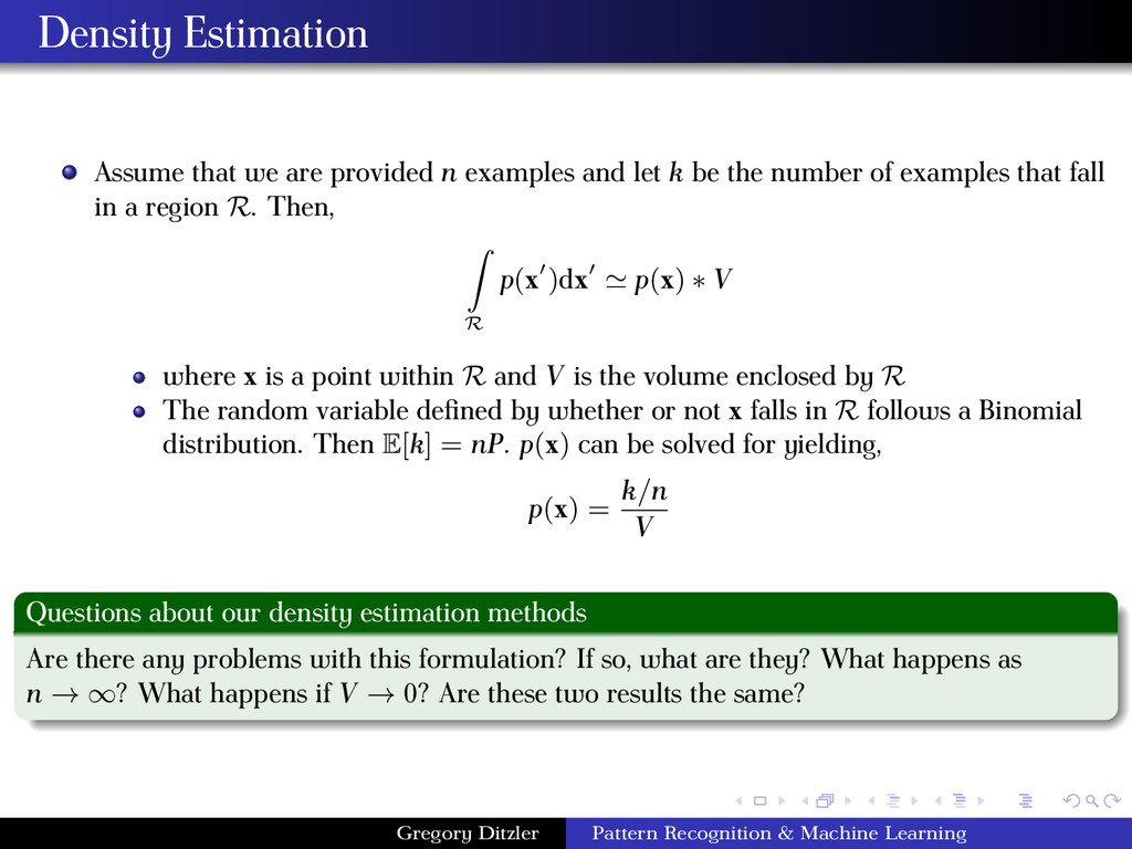
let k be the number of examples that fall in a region R. Then, R p(x )dx p(x) ∗ V where x is a point within R and V is the volume enclosed by R The random variable defined by whether or not x falls in R follows a Binomial distribution. Then E[k] = nP. p(x) can be solved for yielding, p(x) = k/n V Questions about our density estimation methods Are there any problems with this formulation? If so, what are they? What happens as n → ∞? What happens if V → 0? Are these two results the same? Gregory Ditzler Pattern Recognition & Machine Learning
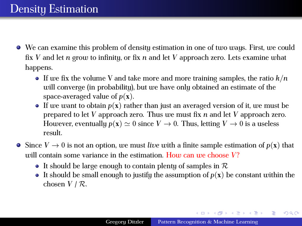
in one of two ways. First, we could fix V and let n grow to infinity, or fix n and let V approach zero. Lets examine what happens. If we fix the volume V and take more and more training samples, the ratio k/n will converge (in probability), but we have only obtained an estimate of the space-averaged value of p(x). If we want to obtain p(x) rather than just an averaged version of it, we must be prepared to let V approach zero. Thus we must fix n and let V approach zero. However, eventually p(x) 0 since V → 0. Thus, letting V → 0 is a useless result. Since V → 0 is not an option, we must live with a finite sample estimation of p(x) that will contain some variance in the estimation. How can we choose V? It should be large enough to contain plenty of samples in R It should be small enough to justify the assumption of p(x) be constant within the chosen V / R. Gregory Ditzler Pattern Recognition & Machine Learning
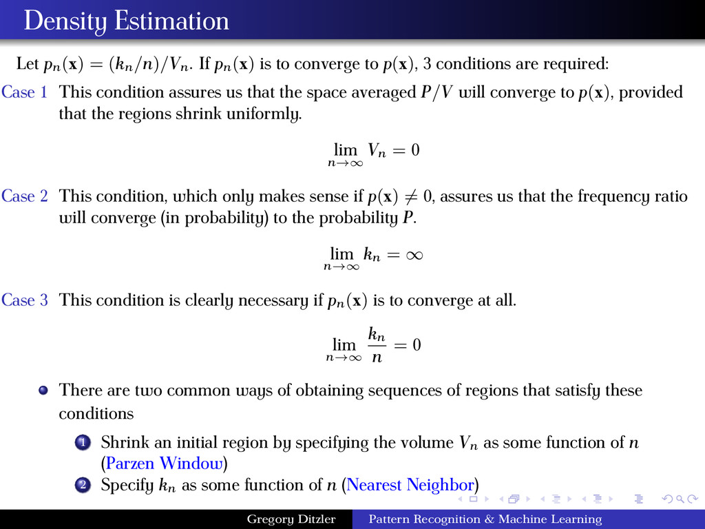
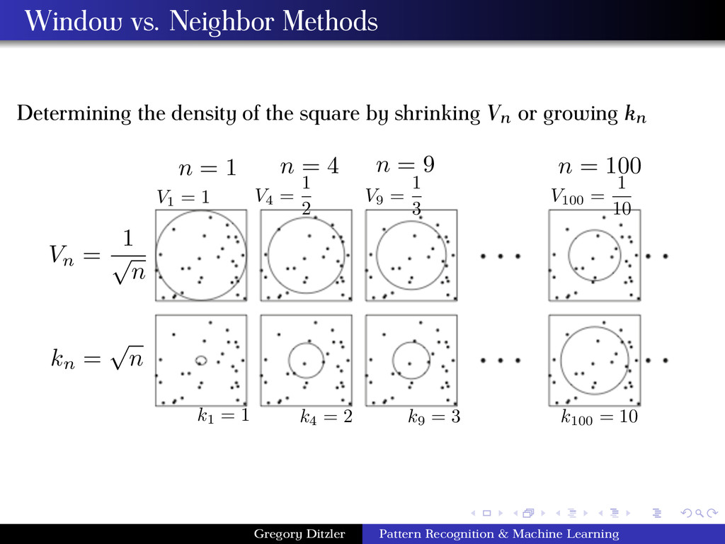
to converge to p(x), 3 conditions are required: Case 1 This condition assures us that the space averaged P/V will converge to p(x), provided that the regions shrink uniformly. lim n→∞ Vn = 0 Case 2 This condition, which only makes sense if p(x) = 0, assures us that the frequency ratio will converge (in probability) to the probability P. lim n→∞ kn = ∞ Case 3 This condition is clearly necessary if pn(x) is to converge at all. lim n→∞ kn n = 0 There are two common ways of obtaining sequences of regions that satisfy these conditions 1 Shrink an initial region by specifying the volume Vn as some function of n (Parzen Window) 2 Specify kn as some function of n (Nearest Neighbor) Gregory Ditzler Pattern Recognition & Machine Learning
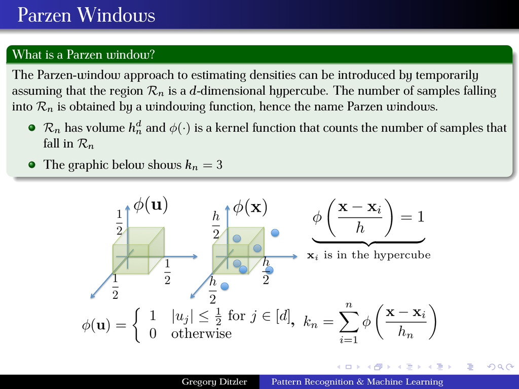
to estimating densities can be introduced by temporarily assuming that the region Rn is a d-dimensional hypercube. The number of samples falling into Rn is obtained by a windowing function, hence the name Parzen windows. Rn has volume hd n and φ(·) is a kernel function that counts the number of samples that fall in Rn The graphic below shows kn = 3 (u) = ⇢ 1 |uj | 1 2 for j 2 [d] 0 otherwise (u) 1 2 1 2 1 2 (x) h 2 h 2 h 2 ✓ x xi h ◆ = 1 | {z } xi is in the hypercube kn = n X i=1 ✓ x xi hn ◆ , Gregory Ditzler Pattern Recognition & Machine Learning
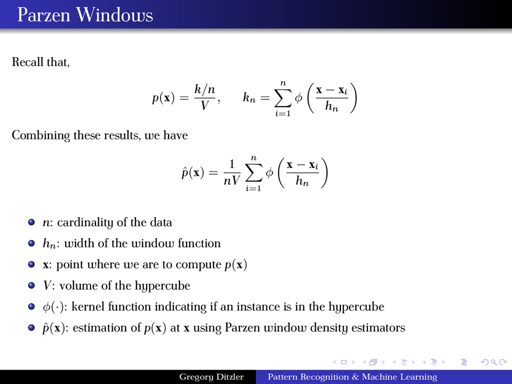
= n i=1 φ x − xi hn Combining these results, we have ˆ p(x) = 1 nV n i=1 φ x − xi hn n: cardinality of the data hn : width of the window function x: point where we are to compute p(x) V: volume of the hypercube φ(·): kernel function indicating if an instance is in the hypercube ˆ p(x): estimation of p(x) at x using Parzen window density estimators Gregory Ditzler Pattern Recognition & Machine Learning
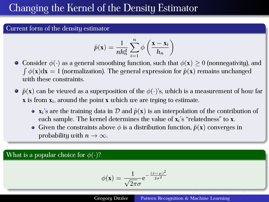
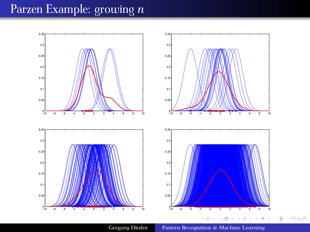
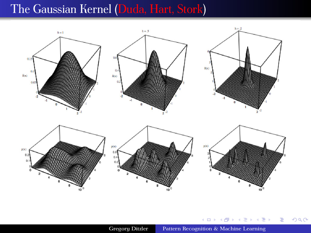
the density estimator ˆ p(x) = 1 nhd n n i=1 φ x − xi hn Consider φ(·) as a general smoothing function, such that φ(x) ≥ 0 (nonnegativity), and φ(x)dx = 1 (normalization). The general expression for ˆ p(x) remains unchanged with these constraints. ˆ p(x) can be viewed as a superposition of the φ(·)’s, which is a measurement of how far x is from xi , around the point x which we are trying to estimate. xi ’s are the training data in D and ˆ p(x) is an interpolation of the contribution of each sample. The kernel determines the value of xi ’s “relatedness” to x. Given the constraints above φ is a distribution function, ˆ p(x) converges in probability with n → ∞. What is a popular choice for φ(·)? φ(x) = 1 √ 2πσ e− (x−µ)2 2σ2 Gregory Ditzler Pattern Recognition & Machine Learning
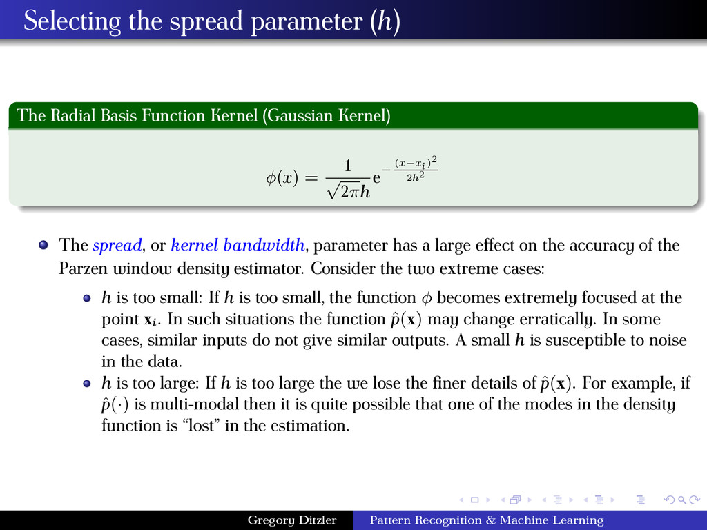
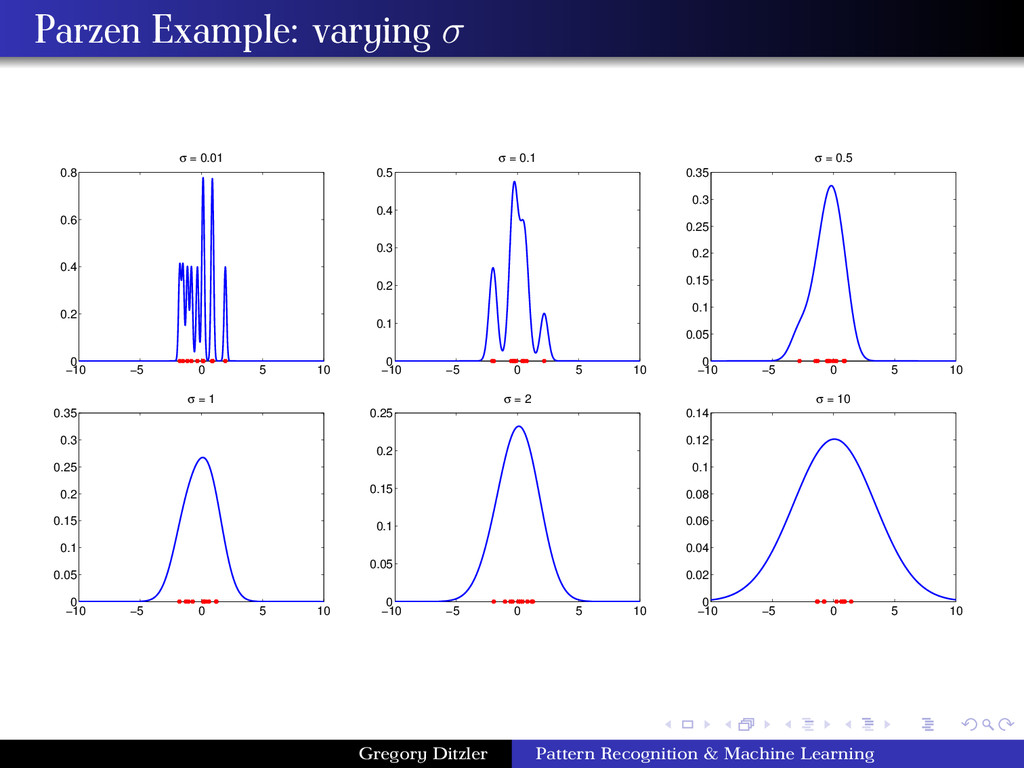
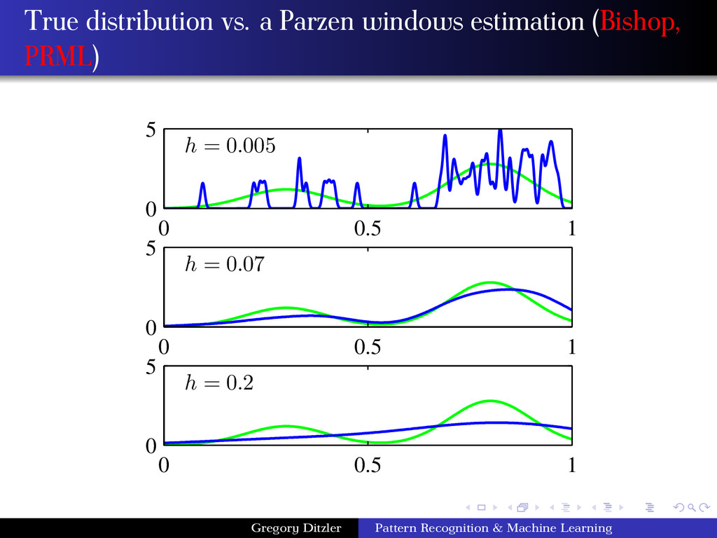
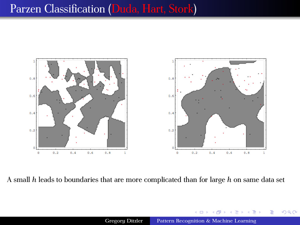
(Gaussian Kernel) φ(x) = 1 √ 2πh e− (x−xi)2 2h2 The spread, or kernel bandwidth, parameter has a large effect on the accuracy of the Parzen window density estimator. Consider the two extreme cases: h is too small: If h is too small, the function φ becomes extremely focused at the point xi . In such situations the function ˆ p(x) may change erratically. In some cases, similar inputs do not give similar outputs. A small h is susceptible to noise in the data. h is too large: If h is too large the we lose the finer details of ˆ p(x). For example, if ˆ p(·) is multi-modal then it is quite possible that one of the modes in the density function is “lost” in the estimation. Gregory Ditzler Pattern Recognition & Machine Learning
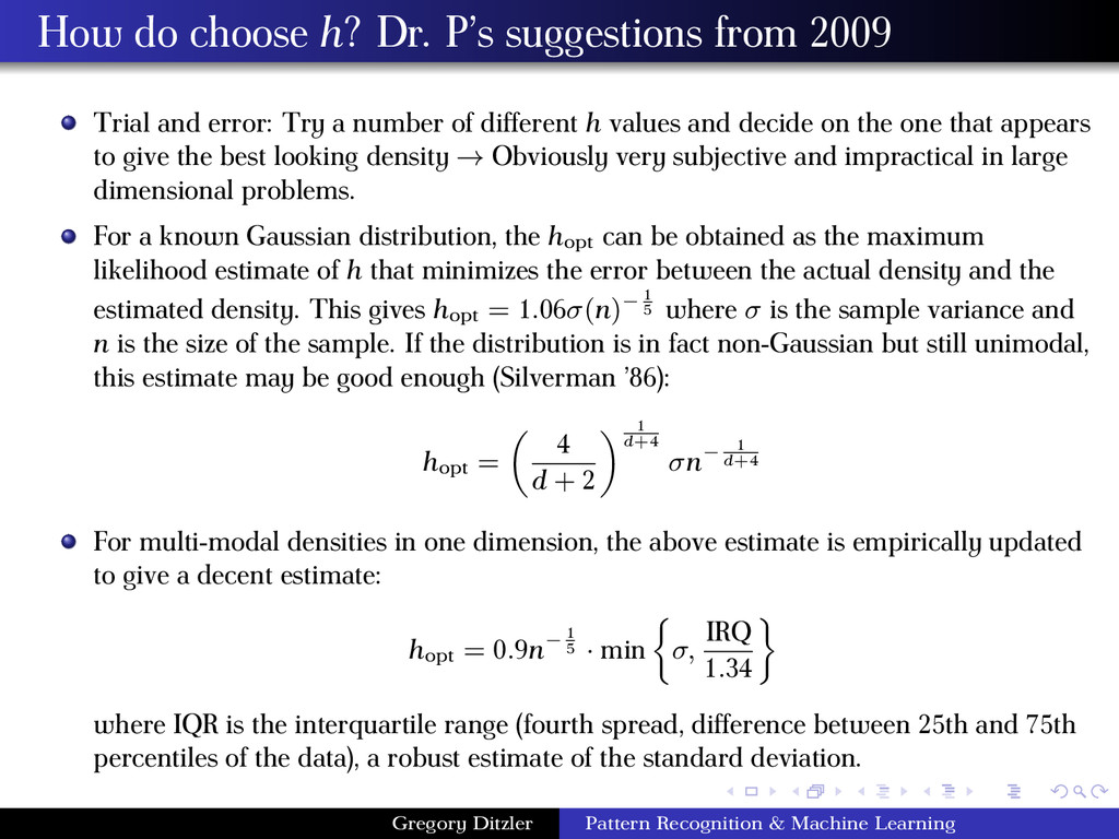
and error: Try a number of different h values and decide on the one that appears to give the best looking density → Obviously very subjective and impractical in large dimensional problems. For a known Gaussian distribution, the hopt can be obtained as the maximum likelihood estimate of h that minimizes the error between the actual density and the estimated density. This gives hopt = 1.06σ(n)− 1 5 where σ is the sample variance and n is the size of the sample. If the distribution is in fact non-Gaussian but still unimodal, this estimate may be good enough (Silverman ’86): hopt = 4 d + 2 1 d+4 σn− 1 d+4 For multi-modal densities in one dimension, the above estimate is empirically updated to give a decent estimate: hopt = 0.9n− 1 5 · min σ, IRQ 1.34 where IQR is the interquartile range (fourth spread, difference between 25th and 75th percentiles of the data), a robust estimate of the standard deviation. Gregory Ditzler Pattern Recognition & Machine Learning
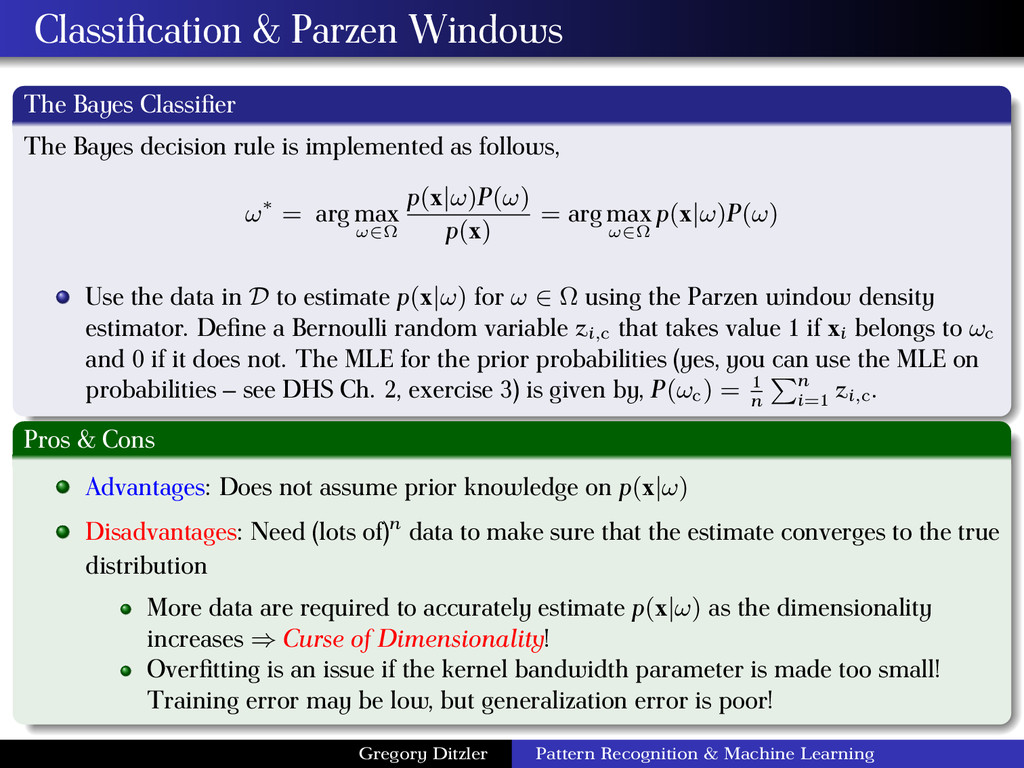
rule is implemented as follows, ω∗ = arg max ω∈Ω p(x|ω)P(ω) p(x) = arg max ω∈Ω p(x|ω)P(ω) Use the data in D to estimate p(x|ω) for ω ∈ Ω using the Parzen window density estimator. Define a Bernoulli random variable zi,c that takes value 1 if xi belongs to ωc and 0 if it does not. The MLE for the prior probabilities (yes, you can use the MLE on probabilities – see DHS Ch. 2, exercise 3) is given by, P(ωc) = 1 n n i=1 zi,c . Pros & Cons Advantages: Does not assume prior knowledge on p(x|ω) Disadvantages: Need (lots of)n data to make sure that the estimate converges to the true distribution More data are required to accurately estimate p(x|ω) as the dimensionality increases ⇒ Curse of Dimensionality! Overfitting is an issue if the kernel bandwidth parameter is made too small! Training error may be low, but generalization error is poor! Gregory Ditzler Pattern Recognition & Machine Learning
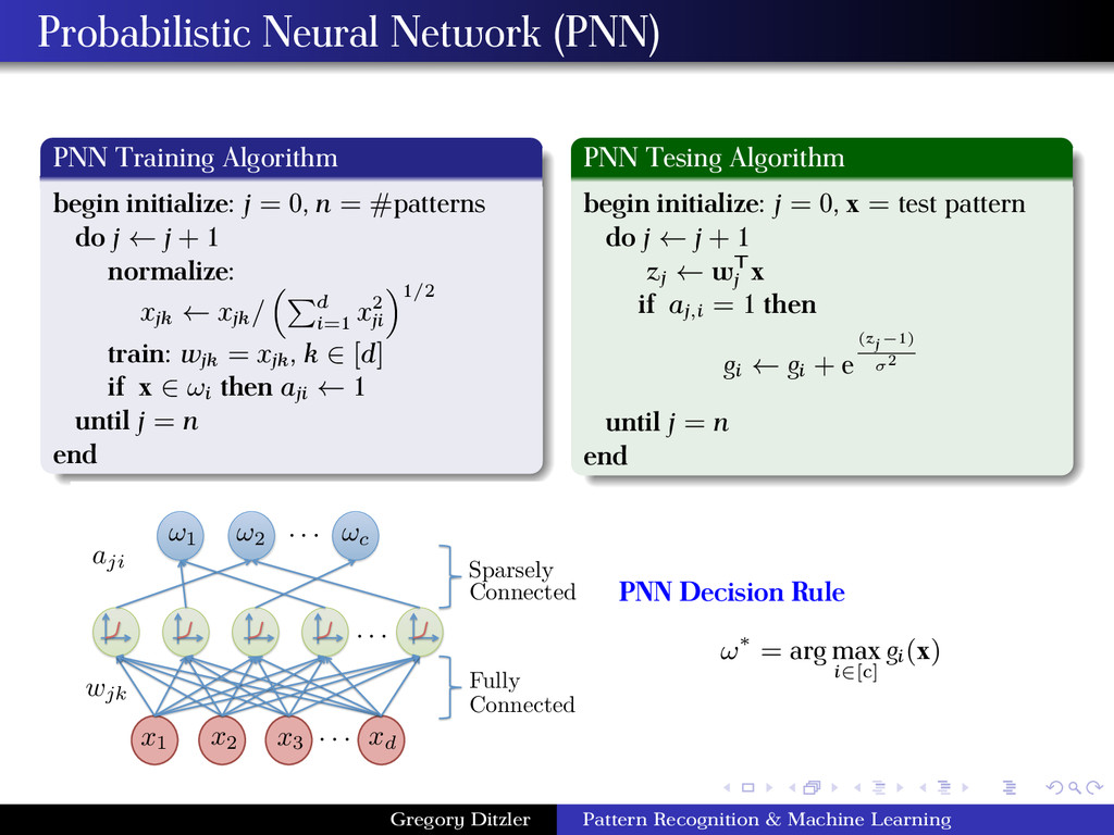
= 0, n = #patterns do j ← j + 1 normalize: xjk ← xjk / d i=1 x2 ji 1/2 train: wjk = xjk , k ∈ [d] if x ∈ ωi then aji ← 1 until j = n end PNN Tesing Algorithm begin initialize: j = 0, x = test pattern do j ← j + 1 zj ← wT j x if aj,i = 1 then gi ← gi + e (zj−1) σ2 until j = n end . . . !1 !2 !c . . . x1 . . . x2 x3 xd Sparsely Connected Connected Fully wjk aji PNN Decision Rule ω∗ = arg max i∈[c] gi(x) Gregory Ditzler Pattern Recognition & Machine Learning
is very fast since the weight vectors are determined by wj = xj . Only a single pass at each example in D is required for learning. This means that the PNN can be used as an online classifier. The space complexity (i.e., how many connections between nodes) is O((n + 1)d). Clearly the storage complexity can be very large. Again, we need to find a reasonable selection of σ (i.e., kernel bandwidth) to avoid over fitting or under fitting the data. The kernel used in the PNN is the radial basis function (RBF). Matlab has a PNN (refer to NEWPNN.m) Gregory Ditzler Pattern Recognition & Machine Learning
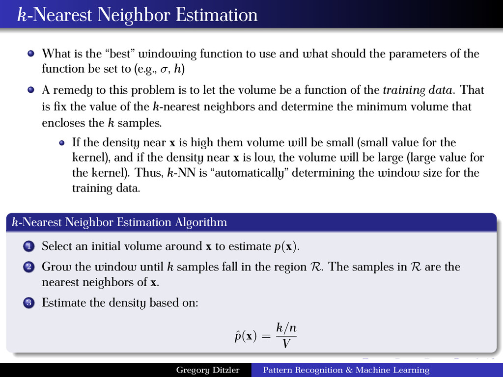
use and what should the parameters of the function be set to (e.g., σ, h) A remedy to this problem is to let the volume be a function of the training data. That is fix the value of the k-nearest neighbors and determine the minimum volume that encloses the k samples. If the density near x is high them volume will be small (small value for the kernel), and if the density near x is low, the volume will be large (large value for the kernel). Thus, k-NN is “automatically” determining the window size for the training data. k-Nearest Neighbor Estimation Algorithm 1 Select an initial volume around x to estimate p(x). 2 Grow the window until k samples fall in the region R. The samples in R are the nearest neighbors of x. 3 Estimate the density based on: ˆ p(x) = k/n V Gregory Ditzler Pattern Recognition & Machine Learning
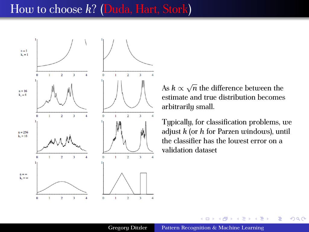
√ n the difference between the estimate and true distribution becomes arbitrarily small. Typically, for classification problems, we adjust k (or h for Parzen windows), until the classifier has the lowest error on a validation dataset Gregory Ditzler Pattern Recognition & Machine Learning
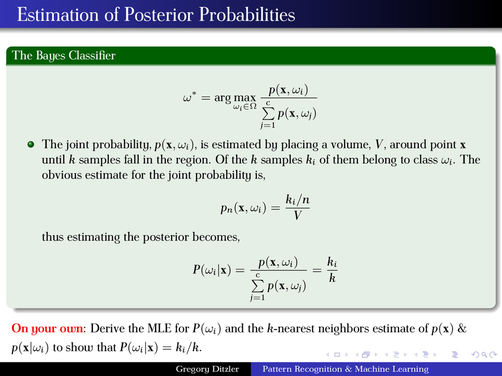
max ωi∈Ω p(x, ωi) c j=1 p(x, ωj ) The joint probability, p(x, ωi), is estimated by placing a volume, V, around point x until k samples fall in the region. Of the k samples ki of them belong to class ωi . The obvious estimate for the joint probability is, pn(x, ωi) = ki/n V thus estimating the posterior becomes, P(ωi|x) = p(x, ωi) c j=1 p(x, ωj ) = ki k On your own: Derive the MLE for P(ωi) and the k-nearest neighbors estimate of p(x) & p(x|ωi) to show that P(ωi|x) = ki/k. Gregory Ditzler Pattern Recognition & Machine Learning
as a lazy learning because there is no “learning” implemented after the training data set. There are no processing steps required before making a prediction other than receiving the training data. Since there is no learning implemented in the k-NN and it is based solely on the training data, k-NN is also called memory based learning, or instance based learning (see Weka’s implementation). Computational cost arises from the testing phase and algorithms require larger memory requirements. Gregory Ditzler Pattern Recognition & Machine Learning
the semester nearly all the algorithms studied assumed that data are labeled. However, supposed we only have access to D = {x1 , . . . , xN } and we need to group them into K sets, or clusters. Intuitively, we might think of a cluster as comprising a group of data points whose inter-point distances are small compared with the distances to points outside of the cluster. Clusters, k = 1, . . . , K are associated with a prototype vector, µk . Our goal is to find the assignment of data samples to clusters such that sum of the squares of the distances of each data point to its closest vector µk , is a minimum. Distortion Minimization min J = min N n=1 K k=1 rnk xn − µk 2 rnk ∈ {0, 1} are binary variables corresponding to whether or not sample n is in cluster k. Another word to describe this variable is a latent variable. Goal: find rnk and µk so as to minimize the distortion. Gregory Ditzler Pattern Recognition & Machine Learning
Algorithm for Finding rnk and µk Initialize µk (e.g., select K instances at random) 1 Minimize J with respect to the rnk , keeping the µk fixed 2 Minimize J with respect to the µk , keeping rnk fixed (repeat until convergence) These two steps updating rnk and updating µk correspond respectively to the E (expectation) and M (maximization) steps of the EM algorithm. Gregory Ditzler Pattern Recognition & Machine Learning
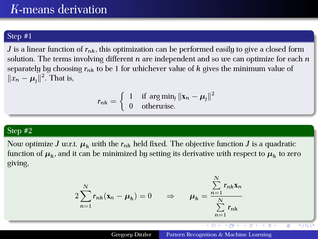
rnk , this optimization can be performed easily to give a closed form solution. The terms involving different n are independent and so we can optimize for each n separately by choosing rnk to be 1 for whichever value of k gives the minimum value of xn − µj 2. That is, rnk = 1 if arg minj xn − µj 2 0 otherwise. Step #2 Now optimize J w.r.t. µk with the rnk held fixed. The objective function J is a quadratic function of µk , and it can be minimized by setting its derivative with respect to µk to zero giving, 2 N n=1 rnk (xn − µk ) = 0 ⇒ µk = N n=1 rnk xn N n=1 rnk Gregory Ditzler Pattern Recognition & Machine Learning
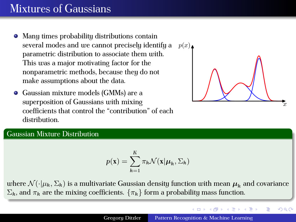
and we cannot precisely identify a parametric distribution to associate them with. This was a major motivating factor for the nonparametric methods, because they do not make assumptions about the data. Gaussian mixture models (GMMs) are a superposition of Gaussians with mixing coefficients that control the “contribution” of each distribution. x p(x) Gaussian Mixture Distribution p(x) = K k=1 πk N(x|µk , Σk ) where N(·|µk , Σk ) is a multivariate Gaussian density function with mean µk and covariance Σk , and πk are the mixing coefficients. {πk } form a probability mass function. Gregory Ditzler Pattern Recognition & Machine Learning
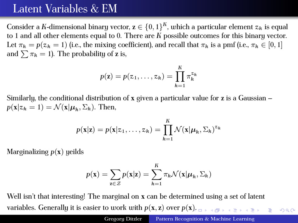
∈ {0, 1}K, which a particular element zk is equal to 1 and all other elements equal to 0. There are K possible outcomes for this binary vector. Let πk = p(zk = 1) (i.e., the mixing coefficient), and recall that πk is a pmf (i.e., πk ∈ [0, 1] and πk = 1). The probability of z is, p(z) = p(z1 , . . . , zk ) = K k=1 πzk k Similarly, the conditional distribution of x given a particular value for z is a Gaussian – p(x|zk = 1) = N(x|µk , Σk ). Then, p(x|z) = p(x|z1 , . . . , zk ) = K k=1 N(x|µk , Σk )zk Marginalizing p(x) yeilds p(x) = z∈Z p(x|z) = K k=1 πk N(x|µk , Σk ) Well isn’t that interesting! The marginal on x can be determined using a set of latent variables. Generally it is easier to work with p(x, z) over p(x). Gregory Ditzler Pattern Recognition & Machine Learning
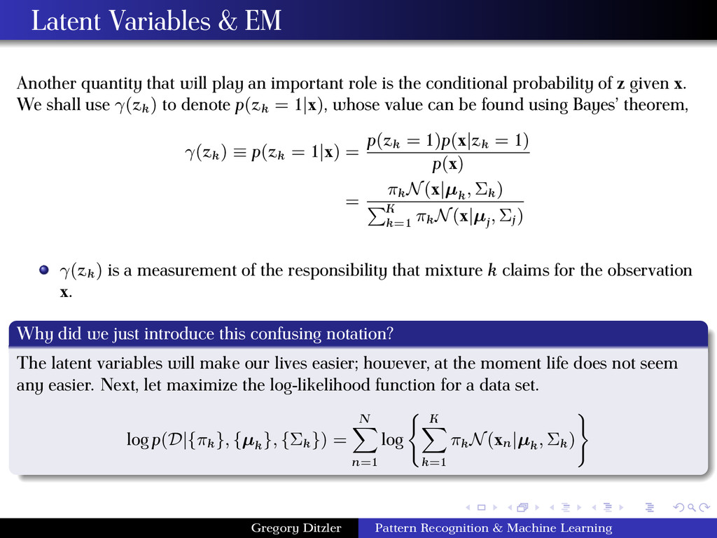
important role is the conditional probability of z given x. We shall use γ(zk ) to denote p(zk = 1|x), whose value can be found using Bayes’ theorem, γ(zk ) ≡ p(zk = 1|x) = p(zk = 1)p(x|zk = 1) p(x) = πk N(x|µk , Σk ) K k=1 πk N(x|µj , Σj ) γ(zk ) is a measurement of the responsibility that mixture k claims for the observation x. Why did we just introduce this confusing notation? The latent variables will make our lives easier; however, at the moment life does not seem any easier. Next, let maximize the log-likelihood function for a data set. log p(D|{πk }, {µk }, {Σk }) = N n=1 log K k=1 πk N(xn|µk , Σk ) Gregory Ditzler Pattern Recognition & Machine Learning
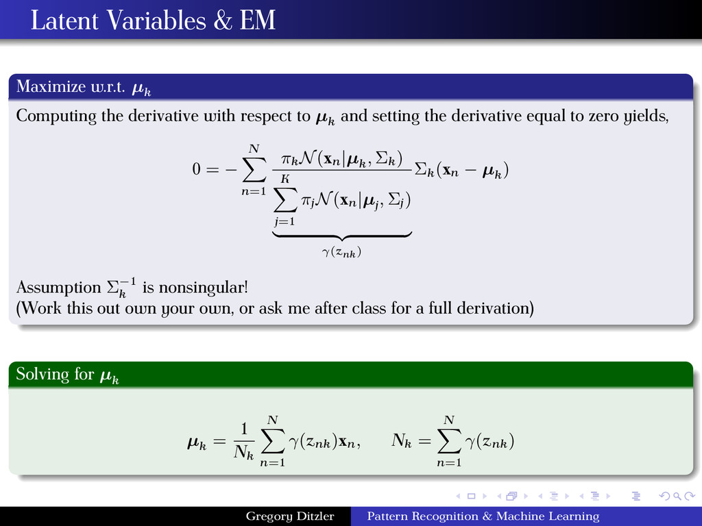
with respect to µk and setting the derivative equal to zero yields, 0 = − N n=1 πk N(xn|µk , Σk ) K j=1 πj N(xn|µj , Σj ) γ(znk) Σk (xn − µk ) Assumption Σ−1 k is nonsingular! (Work this out own your own, or ask me after class for a full derivation) Solving for µk µk = 1 Nk N n=1 γ(znk )xn, Nk = N n=1 γ(znk ) Gregory Ditzler Pattern Recognition & Machine Learning
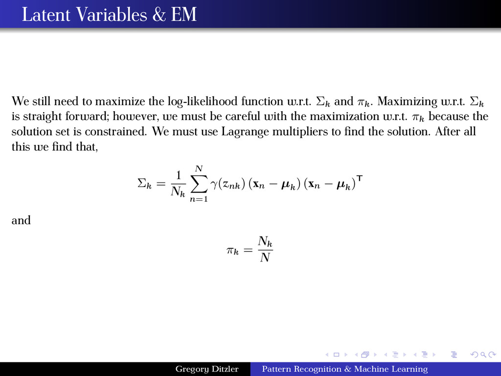
log-likelihood function w.r.t. Σk and πk . Maximizing w.r.t. Σk is straight forward; however, we must be careful with the maximization w.r.t. πk because the solution set is constrained. We must use Lagrange multipliers to find the solution. After all this we find that, Σk = 1 Nk N n=1 γ(znk ) (xn − µk ) (xn − µk )T and πk = Nk N Gregory Ditzler Pattern Recognition & Machine Learning
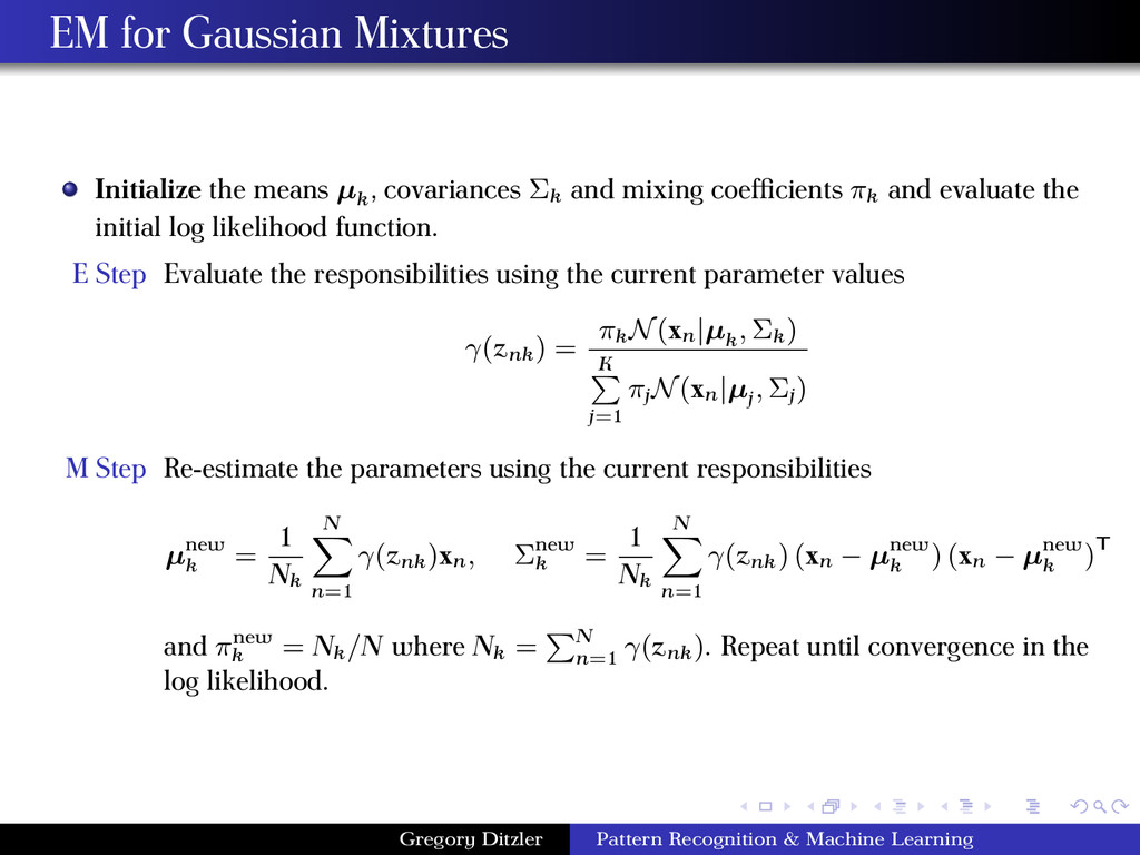
Σk and mixing coefficients πk and evaluate the initial log likelihood function. E Step Evaluate the responsibilities using the current parameter values γ(znk ) = πk N(xn|µk , Σk ) K j=1 πj N(xn|µj , Σj ) M Step Re-estimate the parameters using the current responsibilities µnew k = 1 Nk N n=1 γ(znk )xn, Σnew k = 1 Nk N n=1 γ(znk ) (xn − µnew k ) (xn − µnew k )T and πnew k = Nk /N where Nk = N n=1 γ(znk ). Repeat until convergence in the log likelihood. Gregory Ditzler Pattern Recognition & Machine Learning
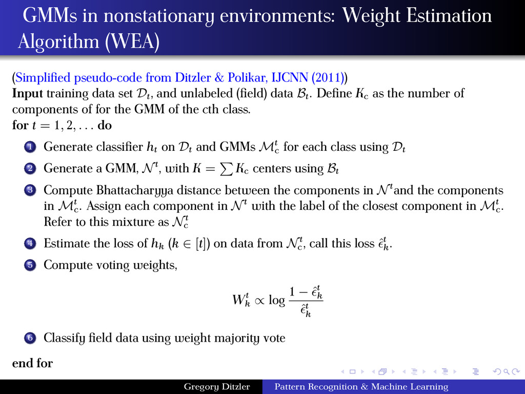
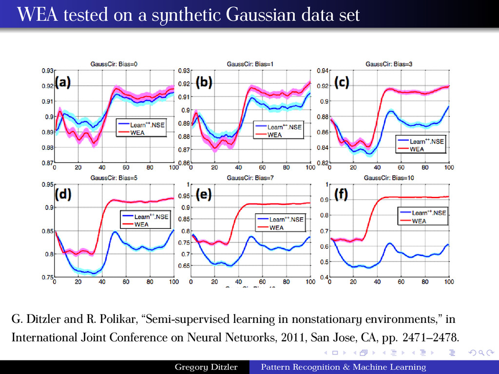
from Ditzler & Polikar, IJCNN (2011)) Input training data set Dt , and unlabeled (field) data Bt . Define Kc as the number of components of for the GMM of the cth class. for t = 1, 2, . . . do 1 Generate classifier ht on Dt and GMMs Mt c for each class using Dt 2 Generate a GMM, Nt, with K = Kc centers using Bt 3 Compute Bhattacharyya distance between the components in Ntand the components in Mt c . Assign each component in Nt with the label of the closest component in Mt c . Refer to this mixture as Nt c 4 Estimate the loss of hk (k ∈ [t]) on data from Nt c , call this loss ˆt k . 5 Compute voting weights, Wt k ∝ log 1 − ˆt k ˆt k 6 Classify field data using weight majority vote end for Gregory Ditzler Pattern Recognition & Machine Learning
and R. Polikar, “Semi-supervised learning in nonstationary environments,” in International Joint Conference on Neural Networks, 2011, San Jose, CA, pp. 2471–2478. Gregory Ditzler Pattern Recognition & Machine Learning
on Demšar’s Journal of Machine Learning Research article on hypothesis testing with multiple classifier over multiple data sets. http://jmlr.csail.mit.edu/papers/volume7/demsar06a/demsar06a.pdf Gregory Ditzler Pattern Recognition & Machine Learning