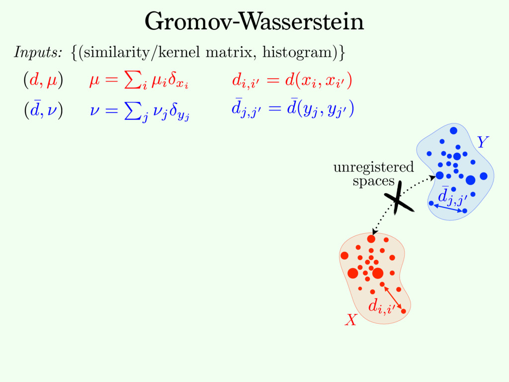
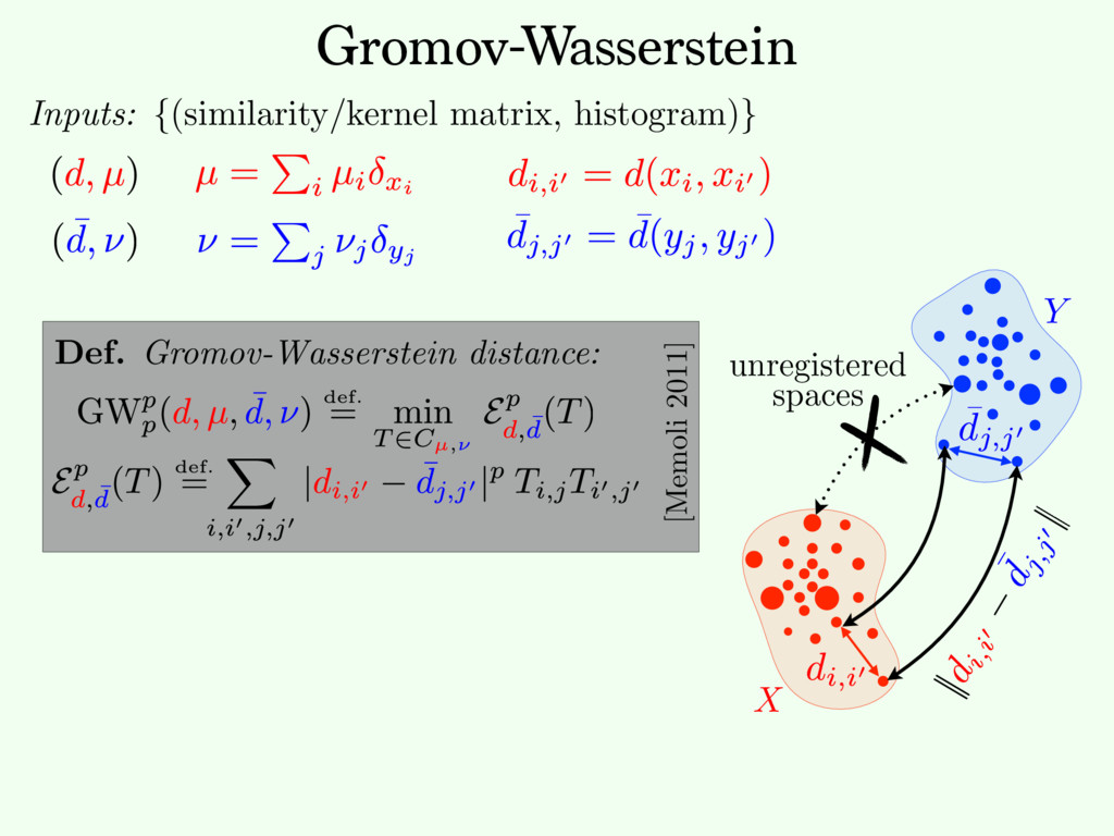
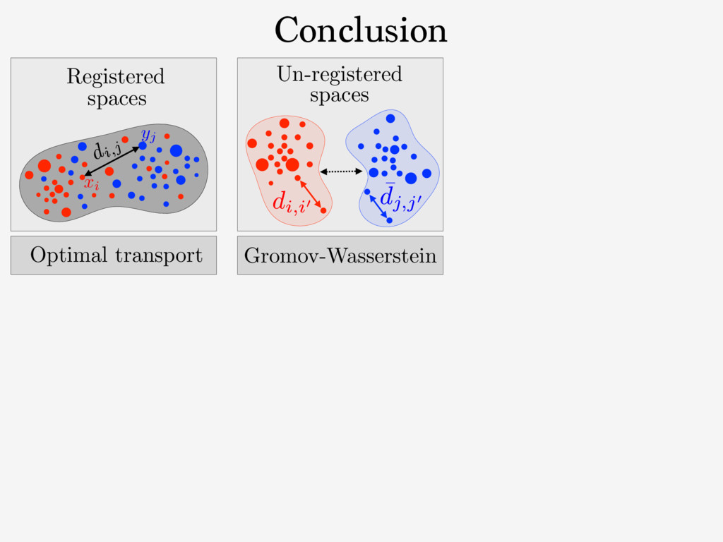
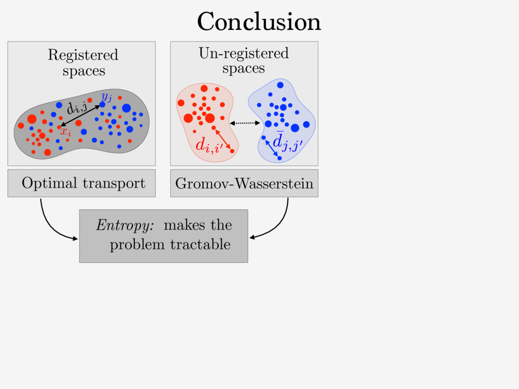
⌃N def. = p 2 R+ N ; P i pi = 1 . The entropy of T 2 RN⇥N + is defined as H ( T ) def. = PN i,j =1 Ti,j (log( Ti,j ) 1) . The set of couplings between histograms p 2 ⌃N1 and q 2 ⌃N2 is Cp,q def. = T 2 ( R +) N1 ⇥N2 ; T1N2 = p, T>1N1 = q . Here, 1N def. = (1 , . . . , 1) > 2 RN . For any tensor L = ( Li,j,k,` )i,j,k,` and matrix ( Ti,j )i,j, we define the tensor- matrix multiplication as L ⌦ T def. = ⇣ X k,` Li,j,k,`Tk,` ⌘ i,j . (1) 2. Gromov-Wasserstein Discrepancy 2.1. Entropic Optimal Transport Optimal transport distances are useful to compare two his- tograms ( p, q ) 2 ⌃N1 ⇥ ⌃N2 defined on the same metric 1 https://github.com/gpeyre/ In our setting, since we learning problems, we d distance matrices, i.e., th does not necessarily sati We define the Gromov- two measured similarity and ( ¯ C, q ) 2 RN2 ⇥N2 ⇥ GW( C, ¯ C, p where EC, ¯ C( T ) The matrix T is a cou which the similarity ma L is some loss function the similarity matrices. the quadratic loss L ( a, the Kullback-Leibler di a log( a/b ) a + b (wh inition (4) of GW ext by (M´ emoli, 2011), sin Entropy: Entropy and Sinkhorn Regularization impact on solution: Def. Regularized OT: [Cuturi NIPS’13] c " T" " repeat: until convergence. initialization: (a, b) (1N1 , 1N2 ) return T = diag(a)K diag(b) Fixed point algorithm: Only matrix/vector multiplications. ! Parallelizable. ! Streams well on GPU.
![[Solomon et al, SIGGRAPH 2015] Generalizations](https://files.speakerdeck.com/presentations/cc7c19cffab64322a50c447fbf56a5c6/slide_9.jpg)
![[Solomon et al, SIGGRAPH 2015] Generalizations [Liereo, Mielke, Savar´ e](https://files.speakerdeck.com/presentations/cc7c19cffab64322a50c447fbf56a5c6/slide_10.jpg)
![[Solomon et al, SIGGRAPH 2015] Generalizations [Liereo, Mielke, Savar´ e](https://files.speakerdeck.com/presentations/cc7c19cffab64322a50c447fbf56a5c6/slide_11.jpg)
![Gromov-Wasserstein Geodesics Def. Gromov-Wasserstein Geodesic Prop. [Sturm 2012]](https://files.speakerdeck.com/presentations/cc7c19cffab64322a50c447fbf56a5c6/slide_32.jpg)