Extending the SSD concept to explore some foundational model limitations: a Bayesian hierarchical approach

Presented at the SETAC Europe 21st Annual Meeting, Milan, Italy (15-19 May 2011)

Transcript

1. Graeme  Hickey1,  Peter  Craig1,  Stuart  Marshall2,  Oliver  Price2,  
   Mathijs  Smit3,  Andy  Hart4,  Robert  LuCk5,  Peter  Chapman2,reGred,  
   Dick  de  Zwart5  
    
   1Department  of  Mathema/cal  Sciences,  Durham  University,  UK  
   2Safety  and  Environmental  Assurance  Centre,  Unilever,  Colworth,  UK  
   3Statoil  ASA,  Trondheim,  Norway  
   4The  Food  and  Environment  Research  Agency,  York,  UK  
   5RIVM,  Bilthoven,  The  Netherlands  
   Extending  the  SSD  Concept  to  Explore  
   Some  Founda/onal  Model  Limita/ons:    
   A  Bayesian  Hierarchical  Approach    
   

   View Slide

2. Species  Sensi/vity  Distribu/ons  (SSDs)  
   log10
   (HC5
   )
   0  
   0.2  
   0.4  
   0.6  
   0.8  
   1  
   -­‐2   -­‐1   0   1   2   3   4  
   %  species  affected  
   log10
   (EC50
   )  of  chemical  for  aqua/c  organisms  
   20
   40
   60
   80
   100
   0
   risk  assessment  
   standard  se]ng  
   

   View Slide

3. All  Models  Are  Wrong…  
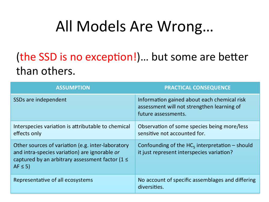
   (the  SSD  is  no  excep/on!)…  but  some  are  beaer  
   than  others.  
   ASSUMPTION   PRACTICAL  CONSEQUENCE  
   SSDs  are  independent   Informa/on  gained  about  each  chemical  risk  
   assessment  will  not  strengthen  learning  of  
   future  assessments.  
   Interspecies  varia/on  is  aaributable  to  chemical  
   effects  only  
   Observa/on  of  some  species  being  more/less  
   sensi/ve  not  accounted  for.  
   Other  sources  of  varia/on  (e.g.  inter-­‐laboratory  
   and  intra-­‐species  varia/on)  are  ignorable  or  
   captured  by  an  arbitrary  assessment  factor  (1  ≤  
   AF  ≤  5)  
   Confounding  of  the  HC5
    interpreta/on  –  should  
   it  just  represent  interspecies  varia/on?  
   Representa/ve  of  all  ecosystems   No  account  of  specific  assemblages  and  differing  
   diversi/es.  
   

   View Slide

4. Hierarchical  Modelling  
   =
   α1  
   σ1
    
   y1j  
    
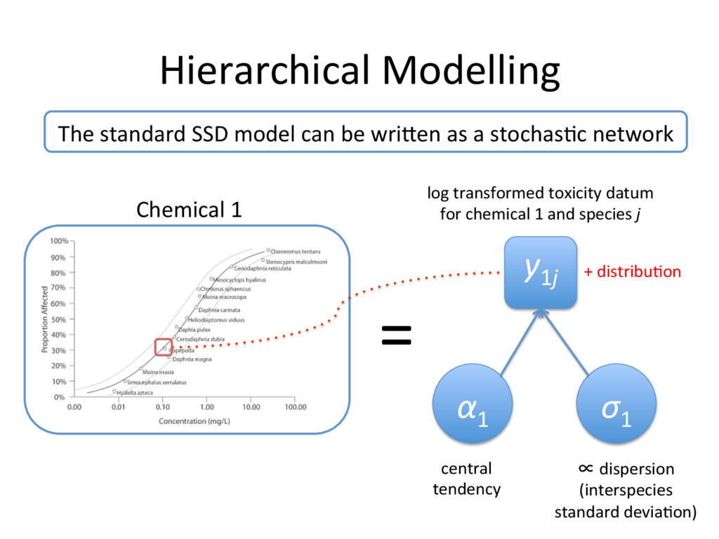
   log  transformed  toxicity  datum  
   for  chemical  1  and  species  j  
   central  
   tendency    
   ˿  dispersion  
   (interspecies  
   standard  devia/on)  
   The  standard  SSD  model  can  be  wriaen  as  a  stochas/c  network  
   +  distribu/on  
   Chemical  1  
   

   View Slide

5. Hierarchical  Modelling  
   α1  
   σ1  
   y1j  
    
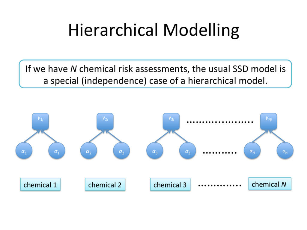
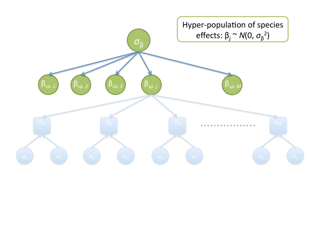
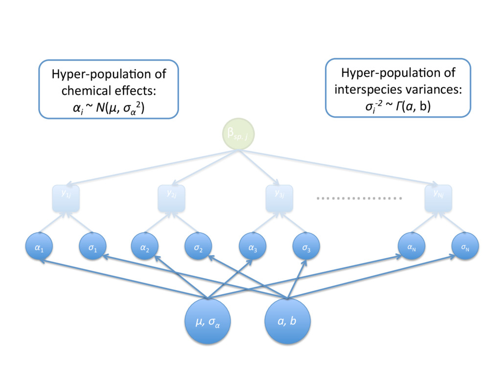
   α2  
   σ2  
   y2j  
    
   α3  
   σ3  
   y3j  
    
   αN  
   σN  
   yNj  
    
   ………...….…..  
   If  we  have  N  chemical  risk  assessments,  the  usual  SSD  model  is  
   a  special  (independence)  case  of  a  hierarchical  model.  
   chemical  1   chemical  2   chemical  3   chemical  N  
   …………..  
   ………..  
   

   View Slide

6. α1  
   σ1  
   y1j  
    
   α2  
   σ2  
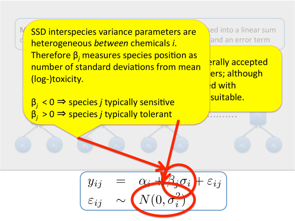
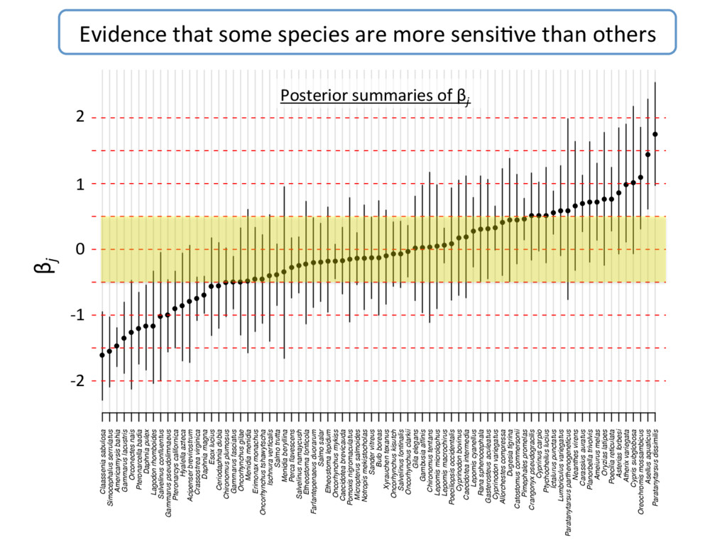
   y2j  
    
   α3  
   σ3  
   y3j  
    
   αN  
   σN  
   yNj  
    
   ……………..  
   βsp.  j  
   Model  Assump8on:  Each  toxicity  value  can  be  decomposed  into  a  linear  sum  
   of  a  chemical  effect,  a  chemical:species  interac/on  effect  and  an  error  term  
   yij = αi + βjσi + εij
   εij
   ∼ N(0, σ2
   i
   )
   Normality  is  generally  accepted  
   by  SSD  prac//oners;  although  
   can  be  subs/tuted  with  
   something  more  suitable.    
   SSD  interspecies  variance  parameters  are  
   heterogeneous  between  chemicals  i.  
   Therefore  βj
    measures  species  posi/on  as  
   number  of  standard  devia/ons  from  mean  
   (log-­‐)toxicity.  
    
   βj
      <  0  ˰  species  j  typically  sensi/ve  
   βj
      >  0  ˰  species  j  typically  tolerant      
   

   View Slide

7. α1  
   σ1  
   y1j  
    
   α2  
   σ2  
   y2j  
    
   α3  
   σ3  
   y3j  
    
   αN  
   σN  
   yNj  
    
   ……………..  
   βsp.  j  
   βsp.  1  
   βsp.  2  
   βsp.  3  
   βsp.  M  
   σβ  
   Hyper-­‐popula/on  of  species  
   effects:  βj
    ~  N(0,  σβ
   2)  
   

   View Slide

8. α1  
   σ1  
   y1j  
    
   α2  
   σ2  
   y2j  
    
   α3  
   σ3  
   y3j  
    
   αN  
   σN  
   yNj  
    
   ……………..  
   βsp.  j  
   μ,  σα  
   a,  b  
   Hyper-­‐popula/on  of  
   chemical  effects:    
   αi
    ~  N(μ,  σα
   2)  
   Hyper-­‐popula/on  of  
   interspecies  variances:    
   σi
   -­‐2  ~  Γ(a,  b)  
   

   View Slide

9. Bayesian  Analysis  
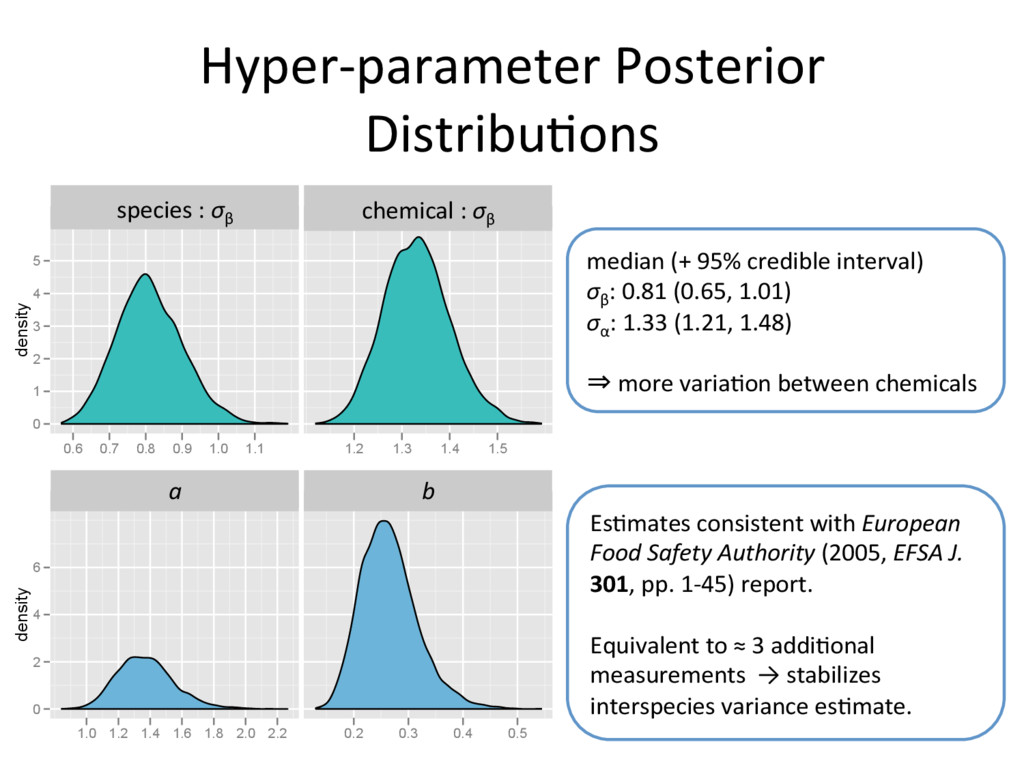
   •  Need  to  ensure  propaga/on  of  >  1st  level  
   uncertainty.  
   •  Update  prior  distribu/ons  about  the  hyper-­‐
   parameters  using  observed  data  to  retrieve  
   posterior  distribu/ons.  
   •  Use  posterior  distribu/ons  to  make  hazard  
   assessment  inferences  for  retrospecGve  and  
   prospecGve  chemical  assessments.  
   

   View Slide

10. Example  
    •  Ecotoxicity  database  extracted  from  the  U.S.  
    EPA  Web-­‐ICE  database.  1600  E(L)C50
     values  
    (lethality  or  immobility)  spanning  201  
    chemicals  (each  with  ni
     ≥  5)  and  77  species.  
     
    hap://www.epa.gov/ceampubl/fchain/webice/  
    •  Prior  distribu/ons  chosen  to  closely  represent  
    ‘ignorance’  (so-­‐called  ‘non-­‐informaGve’).    
    

    View Slide

11. density
    0
    1
    2
    3
    4
    5
    !!
    0.6 0.7 0.8 0.9 1.0 1.1
    !!
    1.2 1.3 1.4 1.5
    Hyper-­‐parameter  Posterior  
    Distribu/ons  
    median  (+  95%  credible  interval)  
    σβ
    :  0.81  (0.65,  1.01)  
    σα
    :  1.33  (1.21,  1.48)  
     
    ˰  more  varia/on  between  chemicals  
    density
    0
    2
    4
    6
    a
    1.0 1.2 1.4 1.6 1.8 2.0 2.2
    b
    0.2 0.3 0.4 0.5
    Es/mates  consistent  with  European  
    Food  Safety  Authority  (2005,  EFSA  J.  
    301,  pp.  1-­‐45)  report.  
     
    Equivalent  to  ≈  3  addi/onal  
    measurements    →  stabilizes  
    interspecies  variance  es/mate.  
    species  :  σβ
      chemical  :  σβ
     
    a   b  
    

    View Slide

12. Posterior distribution summaries of !j
    −2 −1 0 1 2
    Paratanytarsus dissimilis
    Asellus aquaticus
    Oreochromis mossambicus
    Cypris subglobosa
    Atherix variegata
    Asterias forbesi
    Poecilia reticulata
    Oryzias latipes
    Ameiurus melas
    Planorbella trivolvis
    Carassius auratus
    Neanthes virens
    Paratanytarsus parthenogeneticus
    Lumbriculus variegatus
    Ictalurus punctatus
    Ptychocheilus lucius
    Cyprinus carpio
    Crangonyx pseudogracilis
    Pimephales promelas
    Catostomus commersonii
    Dugesia tigrina
    Allorchestes compressa
    Cyprinodon variegatus
    Gasterosteus aculeatus
    Rana sphenocephala
    Lepomis cyanellus
    Caecidotea intermedia
    Cyprinodon bovinus
    Poeciliopsis occidentalis
    Lepomis macrochirus
    Lepomis microlophus
    Chironomus tentans
    Gambusia affinis
    Gila elegans
    Oncorhynchus clarkii
    Salvelinus fontinalis
    Oncorhynchus kisutch
    Xyrauchen texanus
    Bufo boreas
    Sander vitreus
    Notropis mekistocholas
    Micropterus salmoides
    Pomoxis nigromaculatus
    Caecidotea brevicauda
    Oncorhynchus mykiss
    Etheostoma lepidum
    Salmo salar
    Farfantepenaeus duorarum
    Etheostoma fonticola
    Salvelinus namaycush
    Perca flavescens
    Menidia beryllina
    Salmo trutta
    Ischnura verticalis
    Oncorhynchus tshawytscha
    Erimonax monachus
    Menidia menidia
    Oncorhynchus gilae
    Gammarus fasciatus
    Chironomus plumosus
    Ceriodaphnia dubia
    Esox lucius
    Daphnia magna
    Crassostrea virginica
    Acipenser brevirostrum
    Hyalella azteca
    Pteronarcys californica
    Gammarus pseudolimnaeus
    Salvelinus confluentus
    Lagodon rhomboides
    Daphnia pulex
    Pteronarcella badia
    Orconectes nais
    Gammarus lacustris
    Americamysis bahia
    Simocephalus serrulatus
    Claassenia sabulosa
    !
    !
    !
    !
    !
    !
    !
    !
    !
    !
    !
    !
    !
    !
    !
    !
    !
    !
    !
    !
    !
    !
    !
    !
    !
    !
    !
    !
    !
    !
    !
    !
    !
    !
    !
    !
    !
    !
    !
    !
    !
    !
    !
    !
    !
    !
    !
    !
    !
    !
    !
    !
    !
    !
    !
    !
    !
    !
    !
    !
    !
    !
    !
    !
    !
    !
    !
    !
    !
    !
    !
    !
    !
    !
    !
    !
    !
    2  
    1  
    0  
    -­‐1  
    -­‐2  
    Evidence  that  some  species  are  more  sensi/ve  than  others  
    βj  
    Posterior  summaries  of  βj  
    

    View Slide

13. The  Role  of  Taxonomy  
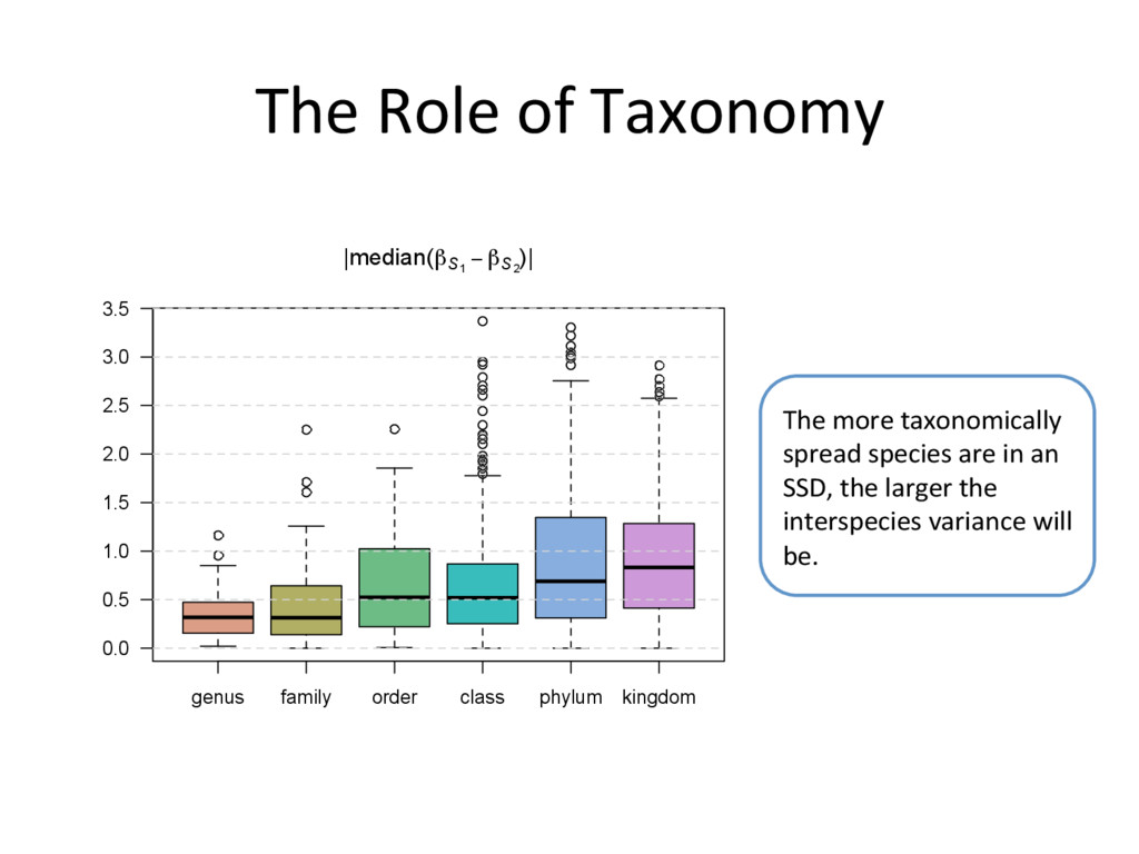
    genus family order class phylum kingdom
    0.0
    0.5
    1.0
    1.5
    2.0
    2.5
    3.0
    3.5
    |median(!S1
    ! !S2
    )|
    The  more  taxonomically  
    spread  species  are  in  an  
    SSD,  the  larger  the  
    interspecies  variance  will  
    be.  
    

    View Slide

14. Posterior  HC5
     Distribu/ons  
    Isofenphos
    !p
    Density
    0.0
    0.2
    0.4
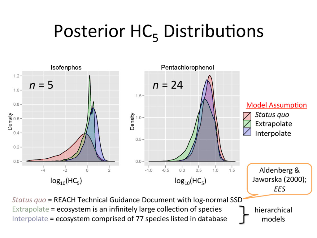
    0.6
    0.8
    1.0
    1.2
    -4 -2 0 2
    Pentachlorophenol
    !p
    Density
    0.0
    0.5
    1.0
    1.5
    -1.0 -0.5 0.0 0.5 1.0 1.5
    Model
    [Default]
    [H: Q = !]
    [H: Q = {!}]
    n  =  5   n  =  24  
    log10
    (HC5
    )   log10
    (HC5
    )  
    Status  quo  
    Extrapolate  
    Interpolate  
    Model  Assump/on  
    Status  quo  =  REACH  Technical  Guidance  Document  with  log-­‐normal  SSD  
    Extrapolate  =  ecosystem  is  an  infinitely  large  collec/on  of  species  
    Interpolate  =  ecosystem  comprised  of  77  species  listed  in  database  
    hierarchical  
    models  
    Aldenberg  &  
    Jaworska  (2000);  
    EES  
    

    View Slide

15. Conclusions  
    •  The  SSD  concept  is  not  defunct!    
    •  Hierarchical  modelling  and  Bayesian  sta/s/cs  
    open  up  the  op/on  for  ‘beaer’  modelling  with  
    transparent  uncertainty  propaga/on.  
    •  Useable  for  mul/ple-­‐hypothesis  tes/ng  and  
    risk  management.  
    

    View Slide

16. Acknowledgements  
    [DATA]  Sandy  Raimondo  and  Mace  Barron  (U.S.  
    EPA,  Gulf  Ecology  Division)  
    [DISCUSSION]  Mick  Hamer  (Syngenta)  and  
    Malyka  Galay-­‐Burgos  (ECETOC)    
    

    View Slide

17. Exis/ng  Hierarchical  Approaches  
    •  Lu]k  &  Aldenberg  (1997),  ET&C  
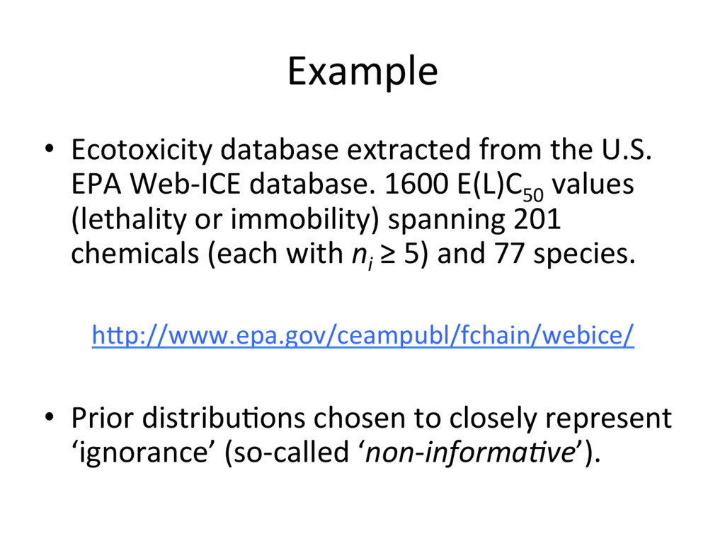
    •  European  Food  Safety  Authority  (2005)  
    •  Jager  et  al.  (2007),  EES  
    •  Morton  (2008),  Environmetrics  
    •  U.S.  EPA  Web-­‐ICE  Program(?)  
    Common  theme:  use  data  from  mul/ple  chemicals  to  
    improve  future  risk  assessments  
    

    View Slide