Lecture slides for POM 1-4

生産管理技術1の講義4のスライドです．

Transcript

1. © Hajime Mizuyama Production & Operations Management #1 @AGU Lec.4: Inventory Control and Management (1) • Factory as a single machine model • Economic order quantity and production lot size • Demand uncertainty and safety stock
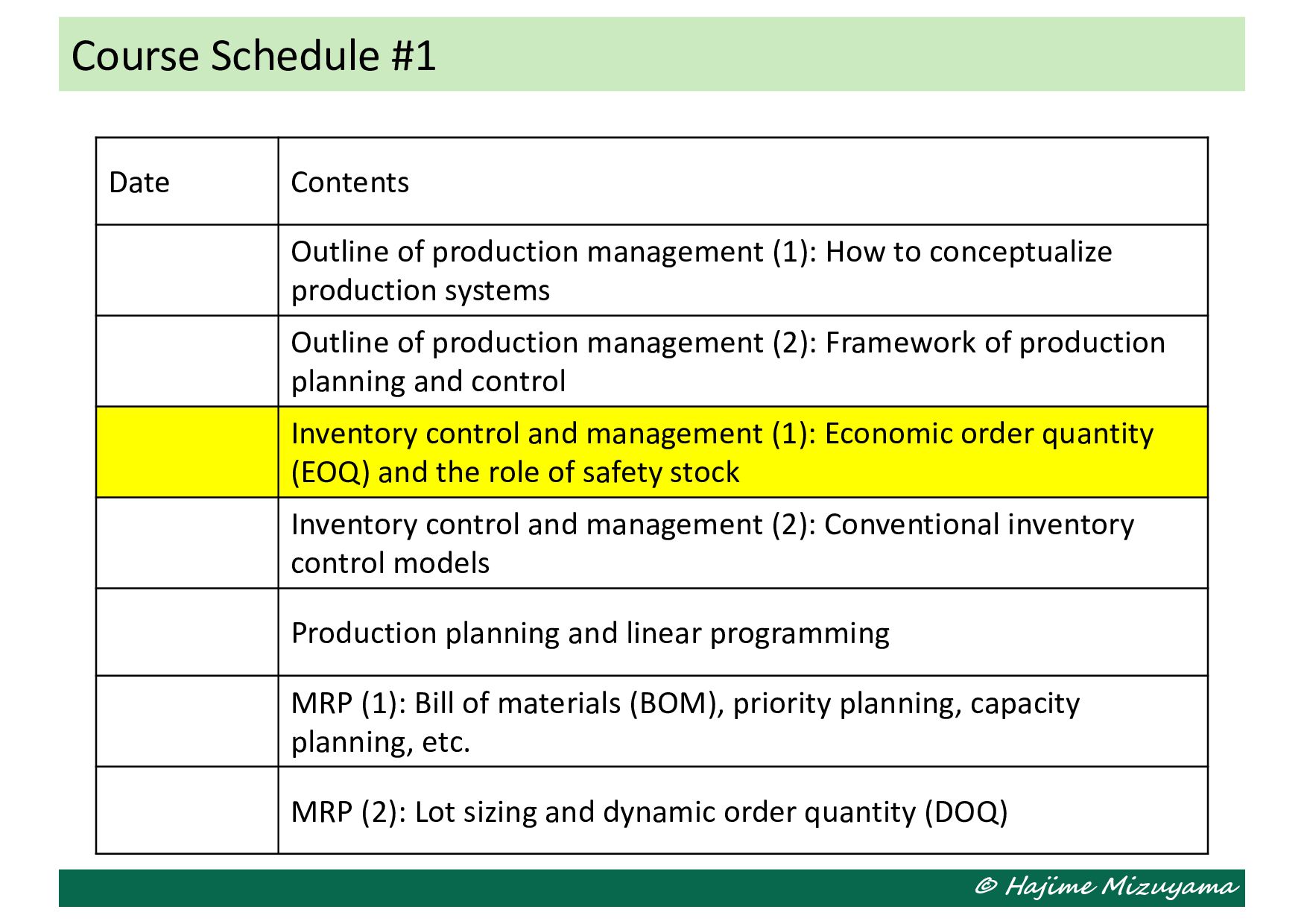
2. © Hajime Mizuyama Course Schedule #1 Date Contents Outline of production management (1): How to conceptualize production systems Outline of production management (2): Framework of production planning and control Inventory control and management (1): Economic order quantity (EOQ) and the role of safety stock Inventory control and management (2): Conventional inventory control models Production planning and linear programming MRP (1): Bill of materials (BOM), priority planning, capacity planning, etc. MRP (2): Lot sizing and dynamic order quantity (DOQ)
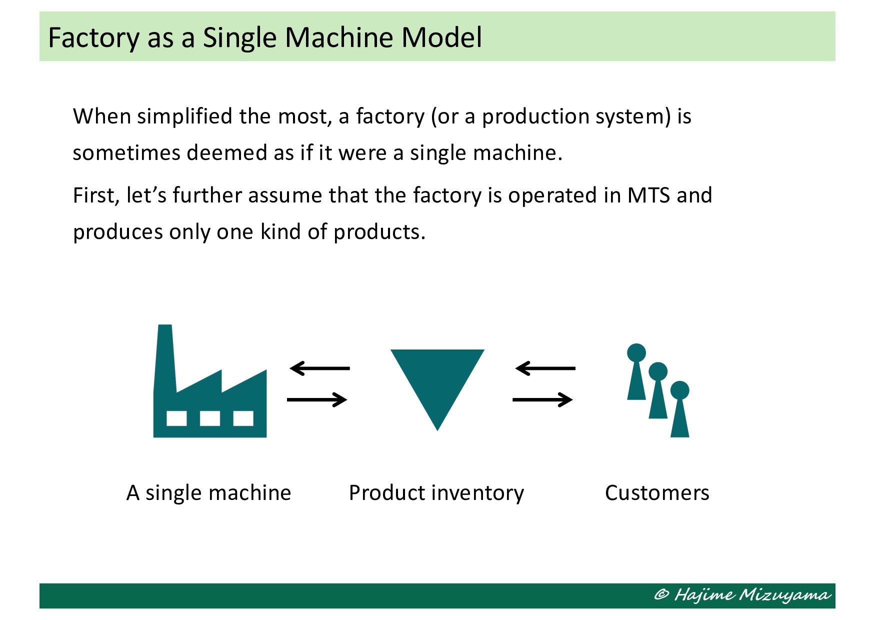
3. © Hajime Mizuyama When simplified the most, a factory (or a production system) is sometimes deemed as if it were a single machine. First, let’s further assume that the factory is operated in MTS and produces only one kind of products. Factory as a Single Machine Model A single machine Product inventory Customers
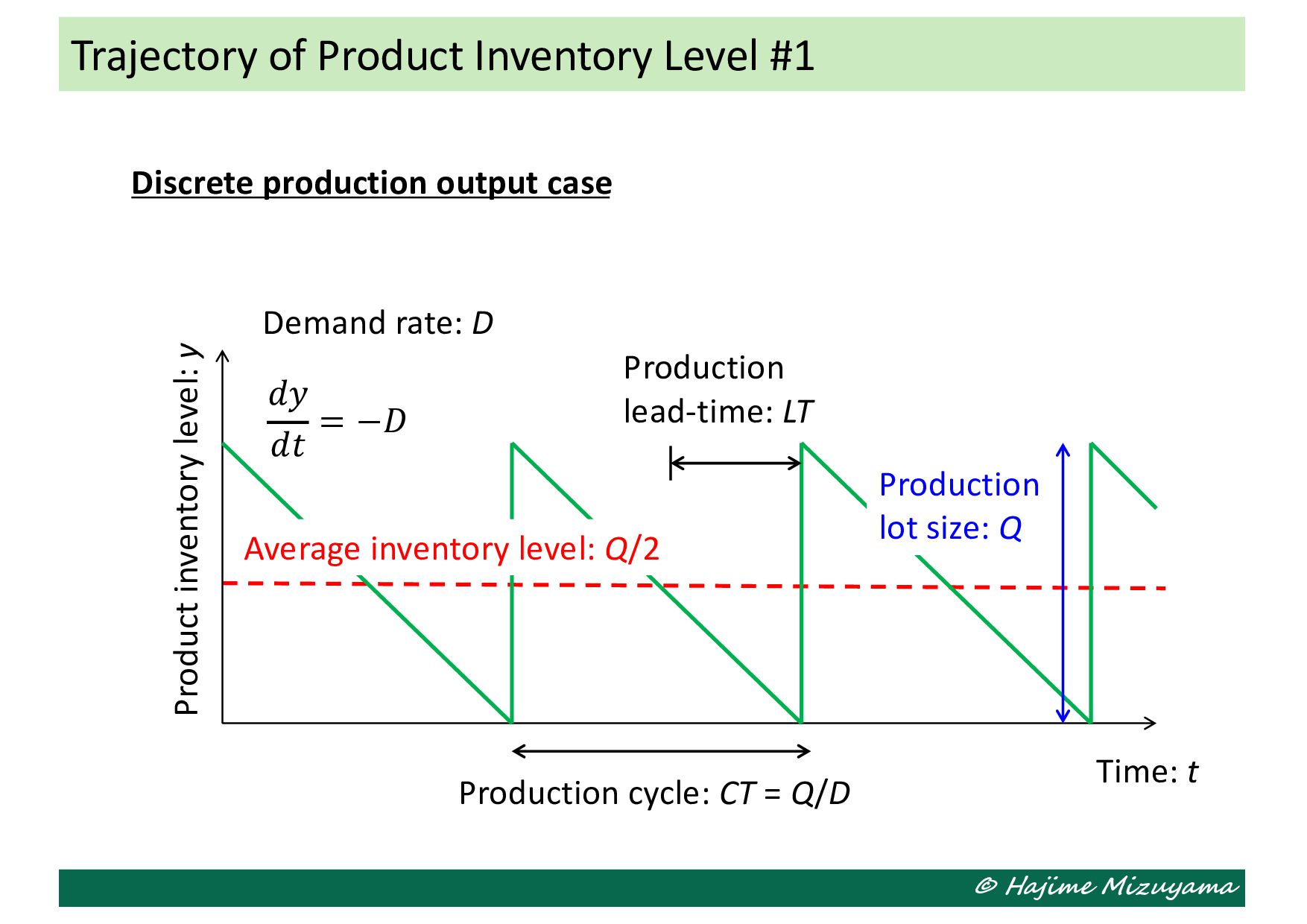
4. © Hajime Mizuyama Trajectory of Product Inventory Level #1 Discrete production output case Product inventory level: y Time: t 𝑑𝑦 𝑑𝑡 = −𝐷 Production lot size: Q Production lead-time: LT Average inventory level: Q/2 Production cycle: CT = Q/D Demand rate: D
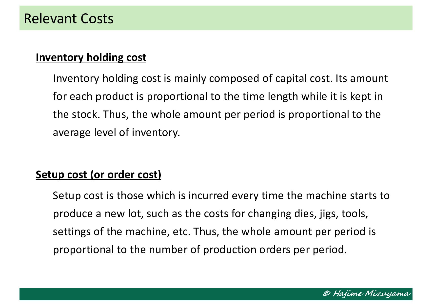
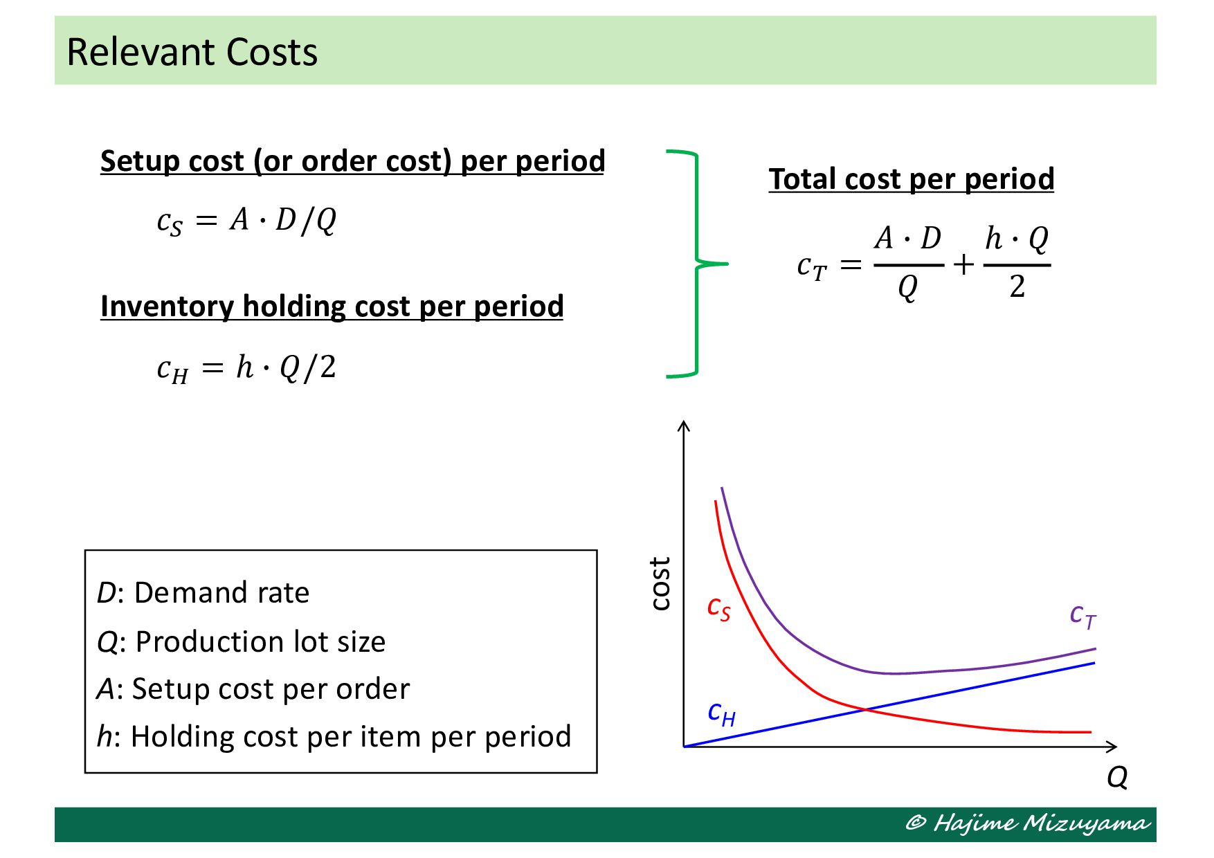
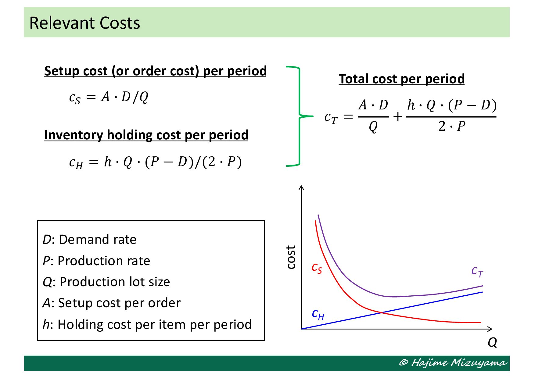
5. © Hajime Mizuyama Inventory holding cost Inventory holding cost is mainly composed of capital cost. Its amount for each product is proportional to the time length while it is kept in the stock. Thus, the whole amount per period is proportional to the average level of inventory. Setup cost (or order cost) Setup cost is those which is incurred every time the machine starts to produce a new lot, such as the costs for changing dies, jigs, tools, settings of the machine, etc. Thus, the whole amount per period is proportional to the number of production orders per period. Relevant Costs
6. © Hajime Mizuyama Setup cost (or order cost) per period 𝑐! = 𝐴 ) 𝐷/𝑄 Inventory holding cost per period 𝑐" = ℎ ) 𝑄/2 Relevant Costs D: Demand rate Q: Production lot size A: Setup cost per order h: Holding cost per item per period Total cost per period 𝑐# = 𝐴 ) 𝐷 𝑄 + ℎ ) 𝑄 2 Q cost cH cS cT
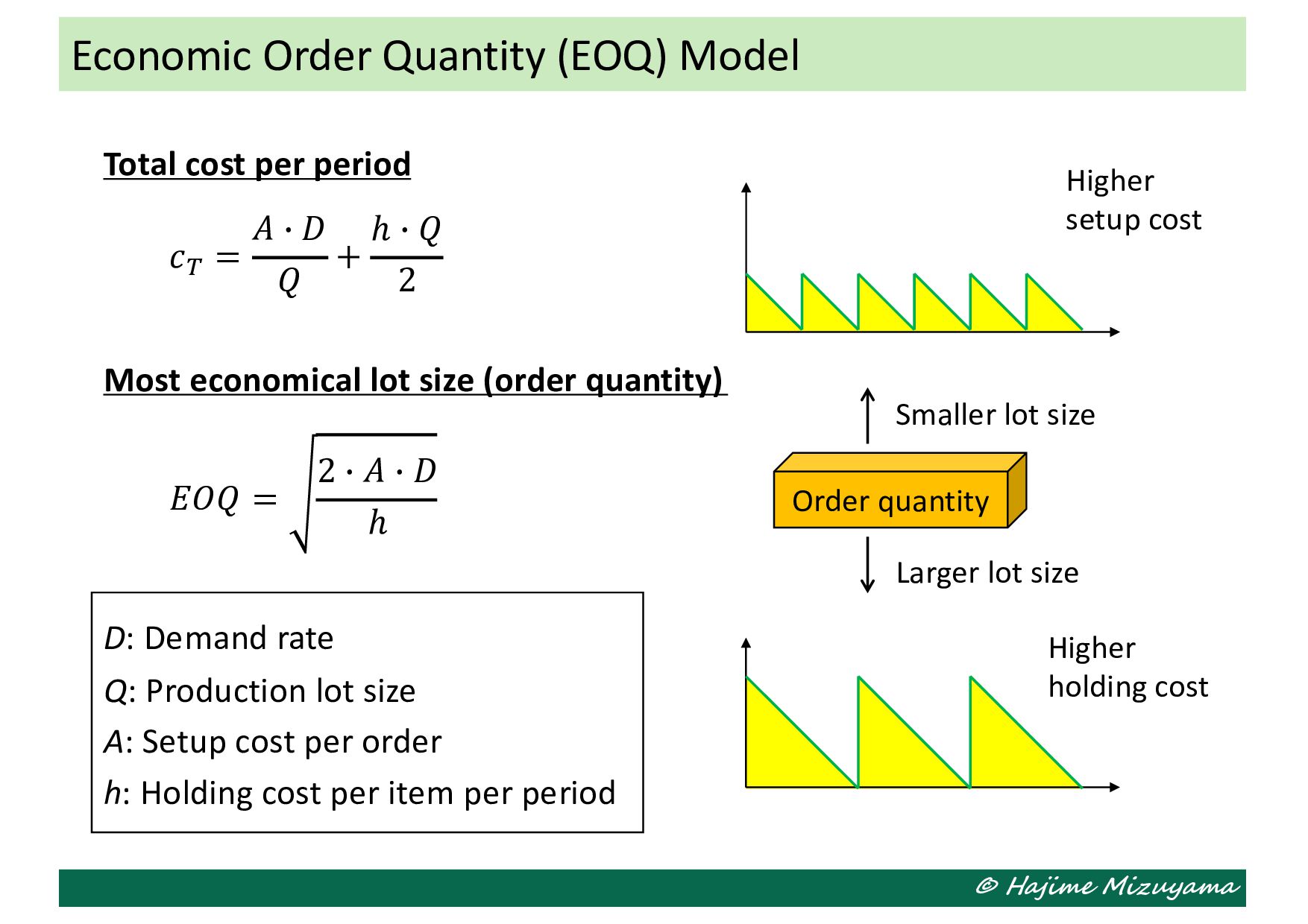
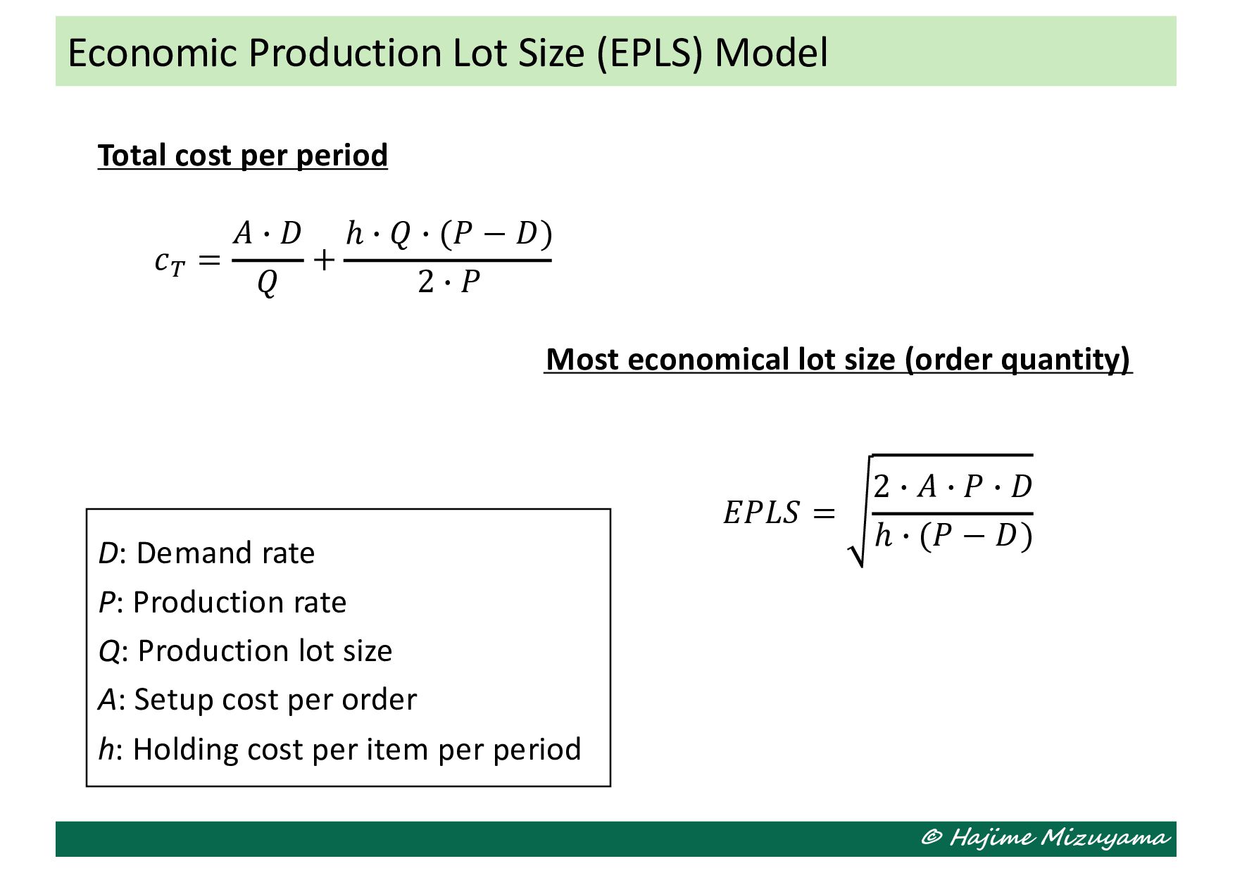
7. © Hajime Mizuyama Total cost per period Most economical lot size (order quantity) Economic Order Quantity (EOQ) Model Order quantity Smaller lot size Larger lot size Higher setup cost Higher holding cost 𝑐# = 𝐴 ) 𝐷 𝑄 + ℎ ) 𝑄 2 𝐸𝑂𝑄 = 2 ) 𝐴 ) 𝐷 ℎ D: Demand rate Q: Production lot size A: Setup cost per order h: Holding cost per item per period
8. © Hajime Mizuyama Numerical Example Demand rate 𝐷 = 500 [items/day] Setup cost per order 𝐴 = 10000 [JPY] Holding cost per item per period ℎ = 10 [JPY/ (item)day)] Economic order quantity (EOQ)
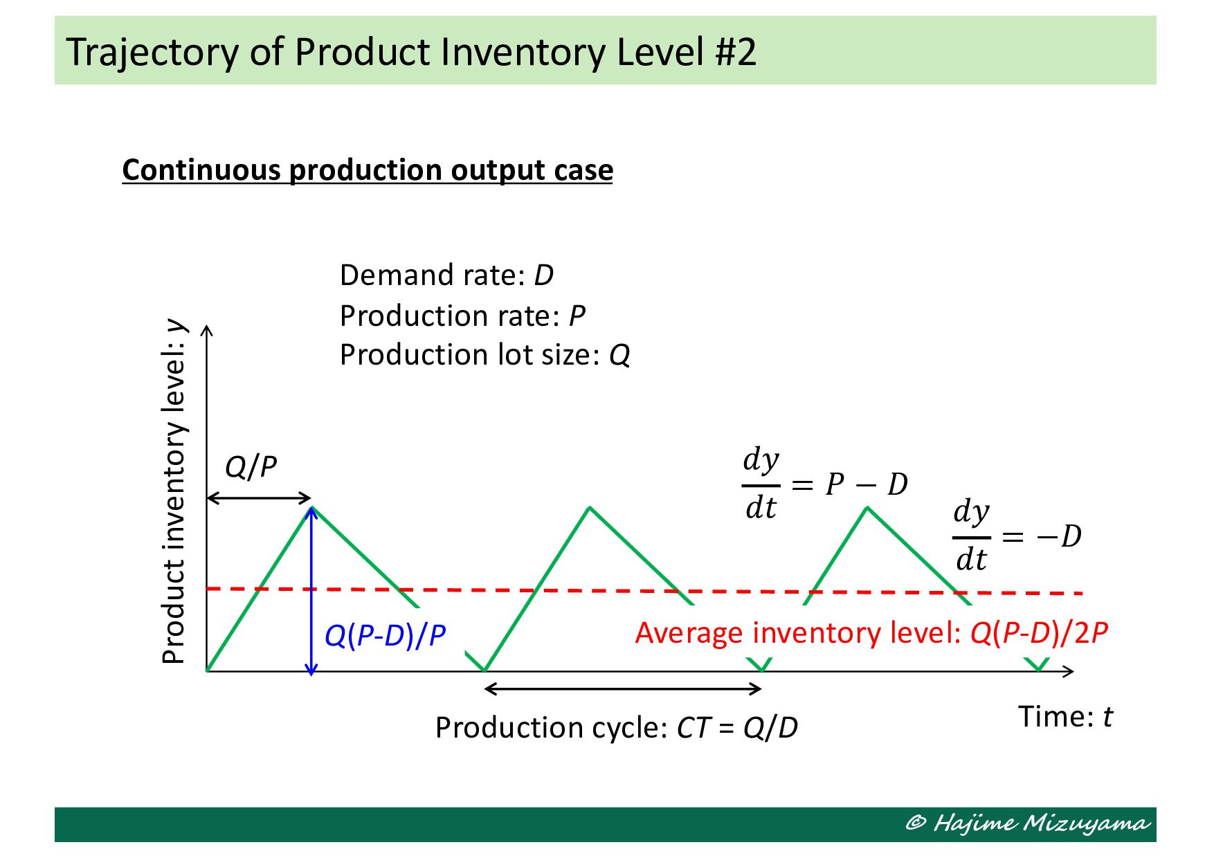
9. © Hajime Mizuyama Trajectory of Product Inventory Level #2 Continuous production output case Product inventory level: y Time: t 𝑑𝑦 𝑑𝑡 = −𝐷 Q/P Production cycle: CT = Q/D Demand rate: D Production rate: P Production lot size: Q 𝑑𝑦 𝑑𝑡 = 𝑃 − 𝐷 Average inventory level: Q(P-D)/2P Q(P-D)/P
10. © Hajime Mizuyama Setup cost (or order cost) per period 𝑐! = 𝐴 ) 𝐷/𝑄 Inventory holding cost per period 𝑐" = ℎ ) 𝑄 ) (𝑃 − 𝐷)/(2 ) 𝑃) Relevant Costs D: Demand rate P: Production rate Q: Production lot size A: Setup cost per order h: Holding cost per item per period Total cost per period 𝑐# = 𝐴 ) 𝐷 𝑄 + ℎ ) 𝑄 ) (𝑃 − 𝐷) 2 ) 𝑃 Q cost cH cS cT
11. © Hajime Mizuyama Total cost per period Most economical lot size (order quantity) Economic Production Lot Size (EPLS) Model 𝐸𝑃𝐿𝑆 = 2 ) 𝐴 ) 𝑃 ) 𝐷 ℎ ) (𝑃 − 𝐷) 𝑐# = 𝐴 ) 𝐷 𝑄 + ℎ ) 𝑄 ) (𝑃 − 𝐷) 2 ) 𝑃 D: Demand rate P: Production rate Q: Production lot size A: Setup cost per order h: Holding cost per item per period
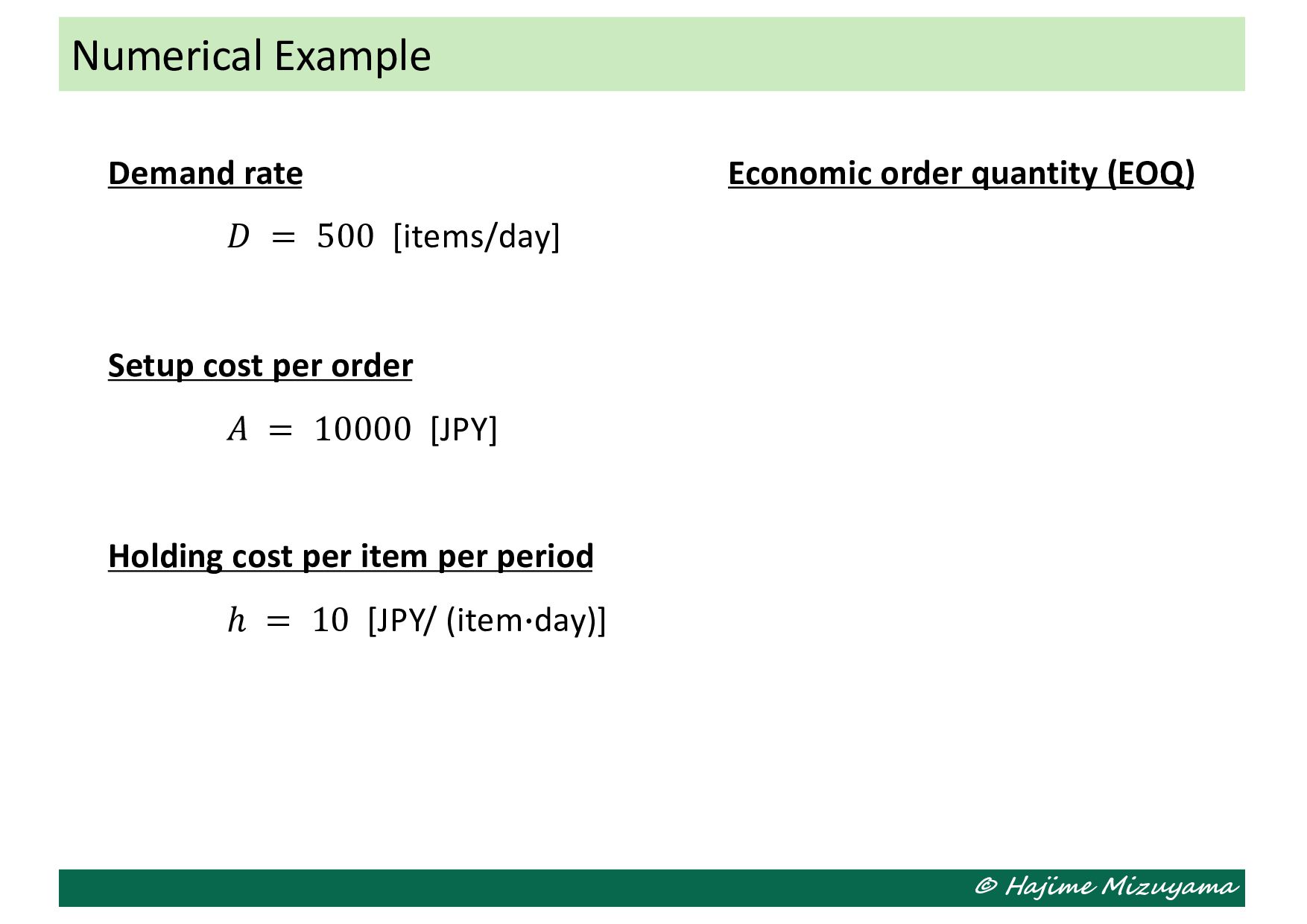
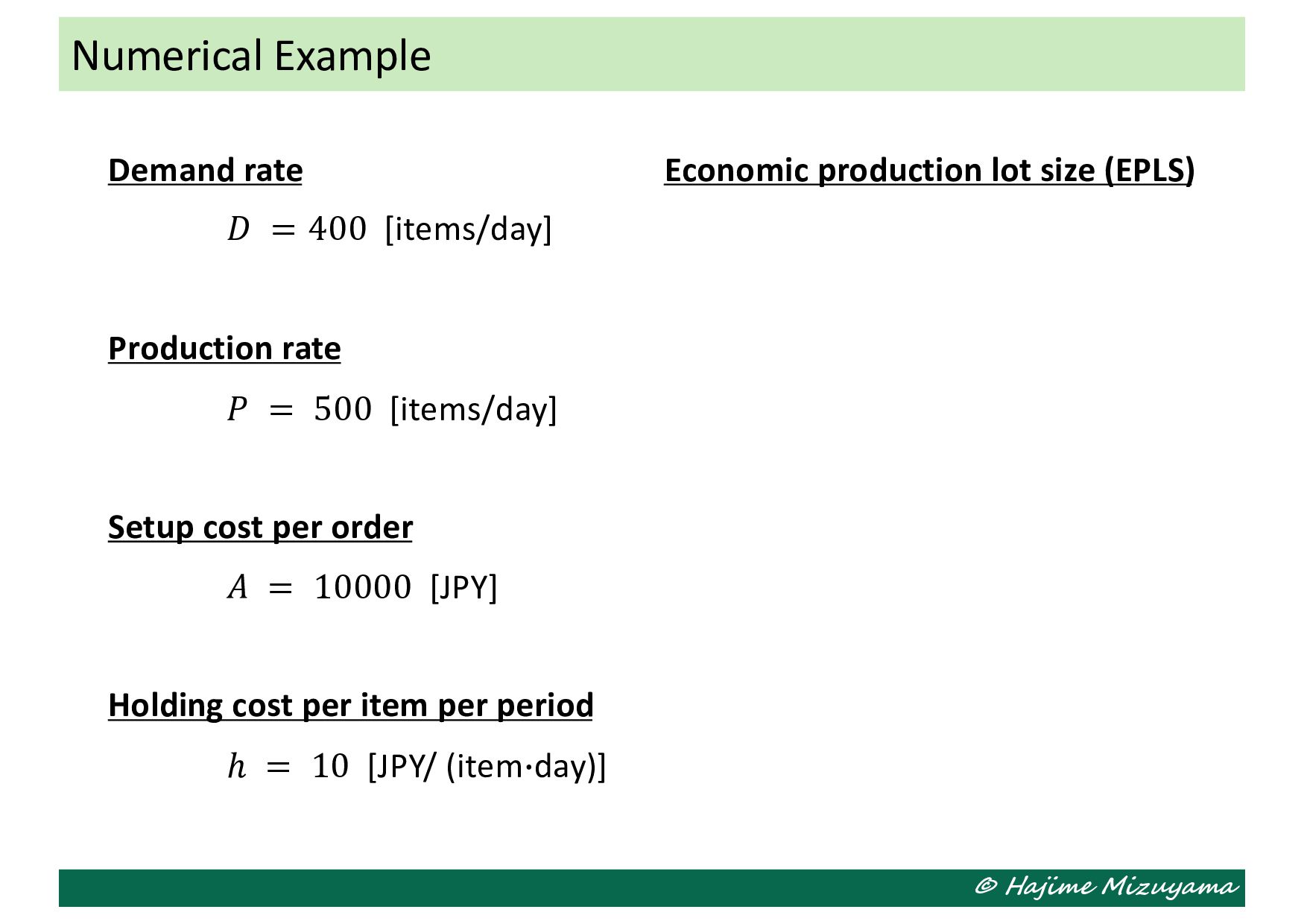
12. © Hajime Mizuyama Numerical Example Demand rate 𝐷 = 400 [items/day] Production rate 𝑃 = 500 [items/day] Setup cost per order 𝐴 = 10000 [JPY] Holding cost per item per period ℎ = 10 [JPY/ (item)day)] Economic production lot size (EPLS)
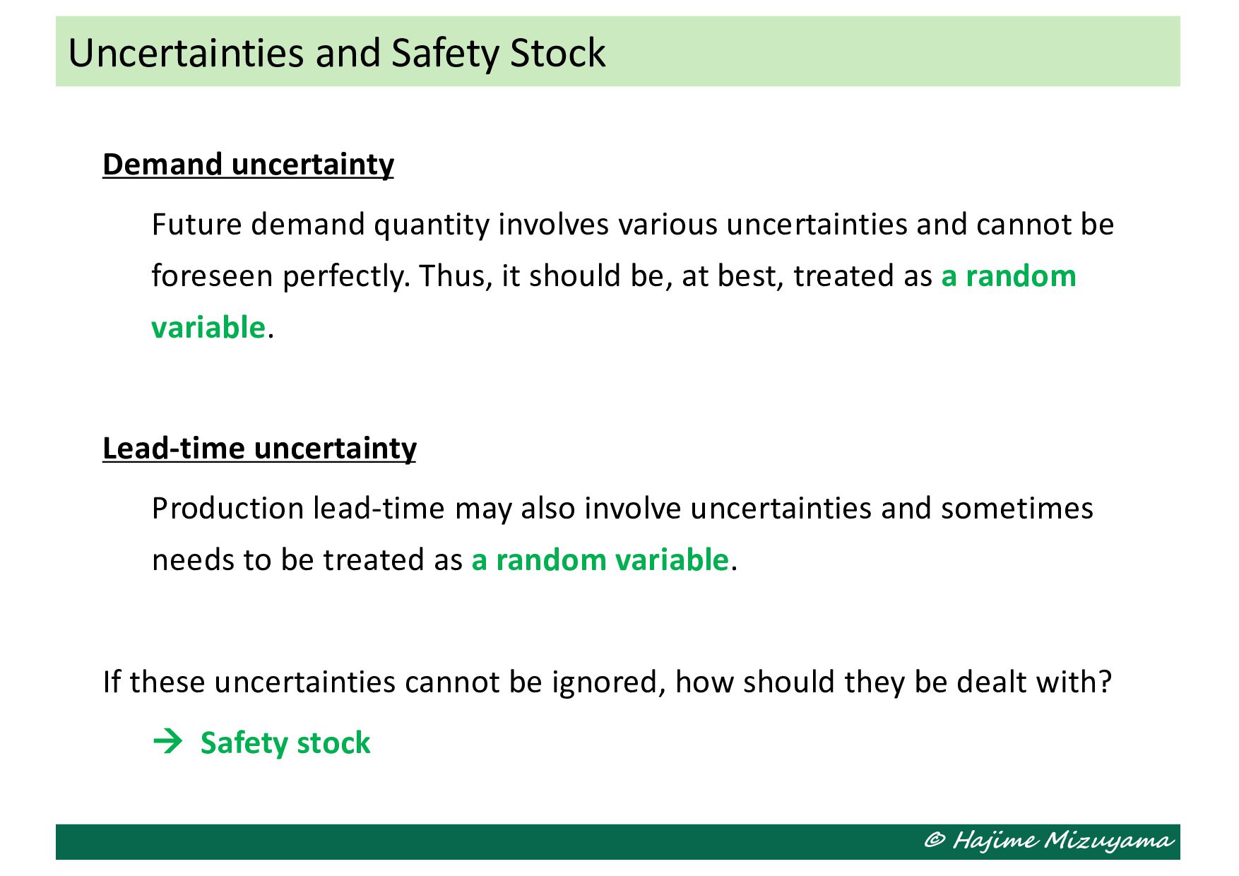
13. © Hajime Mizuyama Demand uncertainty Future demand quantity involves various uncertainties and cannot be foreseen perfectly. Thus, it should be, at best, treated as a random variable. Lead-time uncertainty Production lead-time may also involve uncertainties and sometimes needs to be treated as a random variable. If these uncertainties cannot be ignored, how should they be dealt with? à Safety stock Uncertainties and Safety Stock
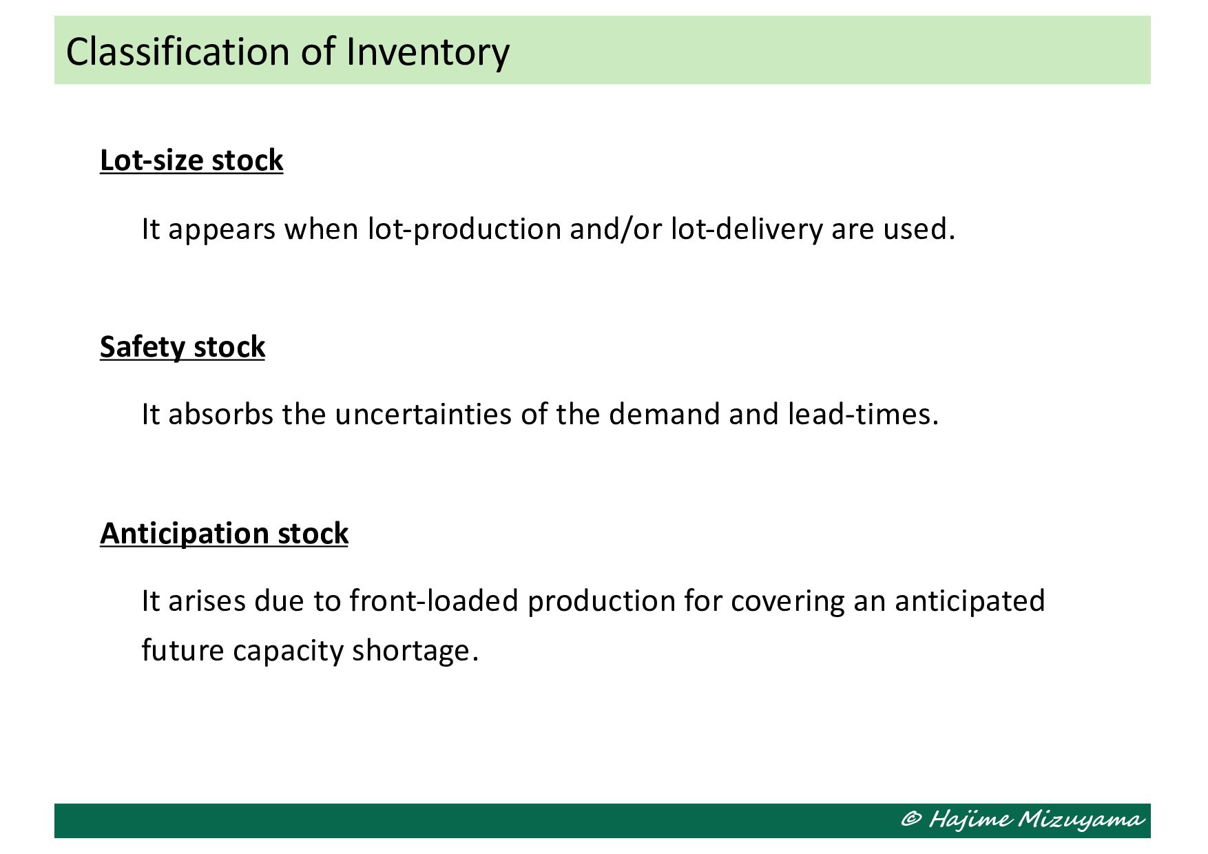
14. © Hajime Mizuyama Lot-size stock It appears when lot-production and/or lot-delivery are used. Safety stock It absorbs the uncertainties of the demand and lead-times. Anticipation stock It arises due to front-loaded production for covering an anticipated future capacity shortage. Classification of Inventory
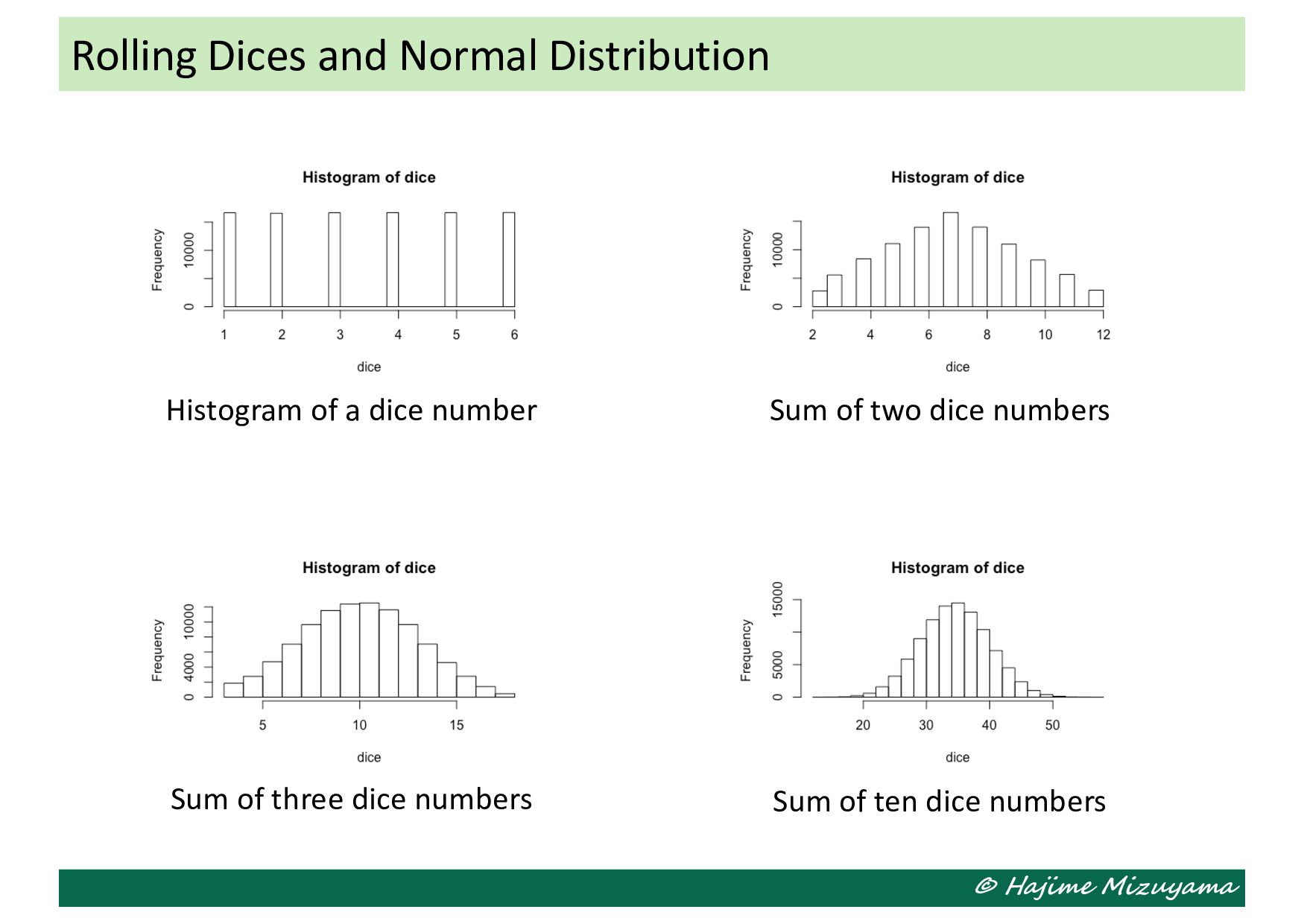
15. © Hajime Mizuyama Random variable • A variable whose value cannot be specified for sure before realization and is only known by its probability distribution, or parameters like mean, variance, etc. • A familiar example would be the number shown on a rolled dice. Normal (Gaussian) distribution • If a lot of independent random variables are summed up, the total will follow this distribution, which is used for various errors and noises. Additivity of variances • The variance of the sum of independent random variables will be the sum of their variances. Additivity of Variance
16. © Hajime Mizuyama Rolling Dices and Normal Distribution Histogram of a dice number Sum of two dice numbers Sum of three dice numbers Sum of ten dice numbers
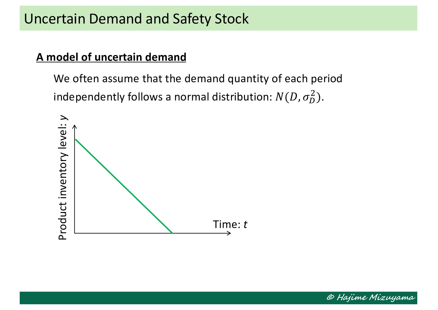
17. © Hajime Mizuyama A model of uncertain demand We often assume that the demand quantity of each period independently follows a normal distribution: 𝑁(𝐷, 𝜎$ %). Uncertain Demand and Safety Stock Product inventory level: y Time: t
18. © Hajime Mizuyama A model of uncertain demand We often assume that the demand quantity of each period independently follows a normal distribution: 𝑁(𝐷, 𝜎$ %). Uncertain Demand and Safety Stock Product inventory level: y Time: t • Backorder à Penalty • Stockout à Opportunity loss Stockout probability The probability that stockout will be caused in each cycle. Service level 1 - Stockout probability
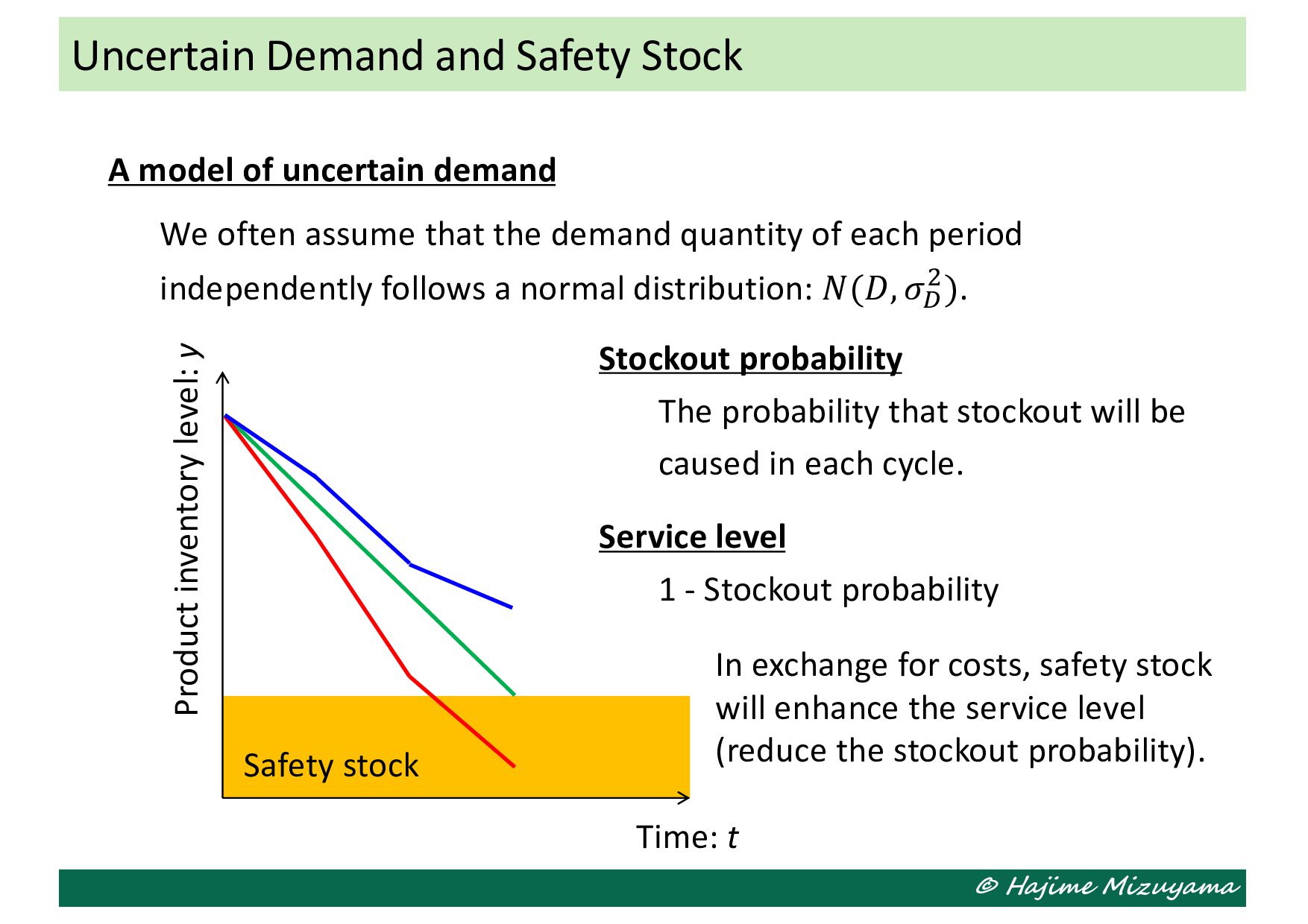
19. © Hajime Mizuyama A model of uncertain demand We often assume that the demand quantity of each period independently follows a normal distribution: 𝑁(𝐷, 𝜎$ %). Uncertain Demand and Safety Stock Product inventory level: y Time: t Stockout probability The probability that stockout will be caused in each cycle. Service level 1 - Stockout probability Safety stock In exchange for costs, safety stock will enhance the service level (reduce the stockout probability).
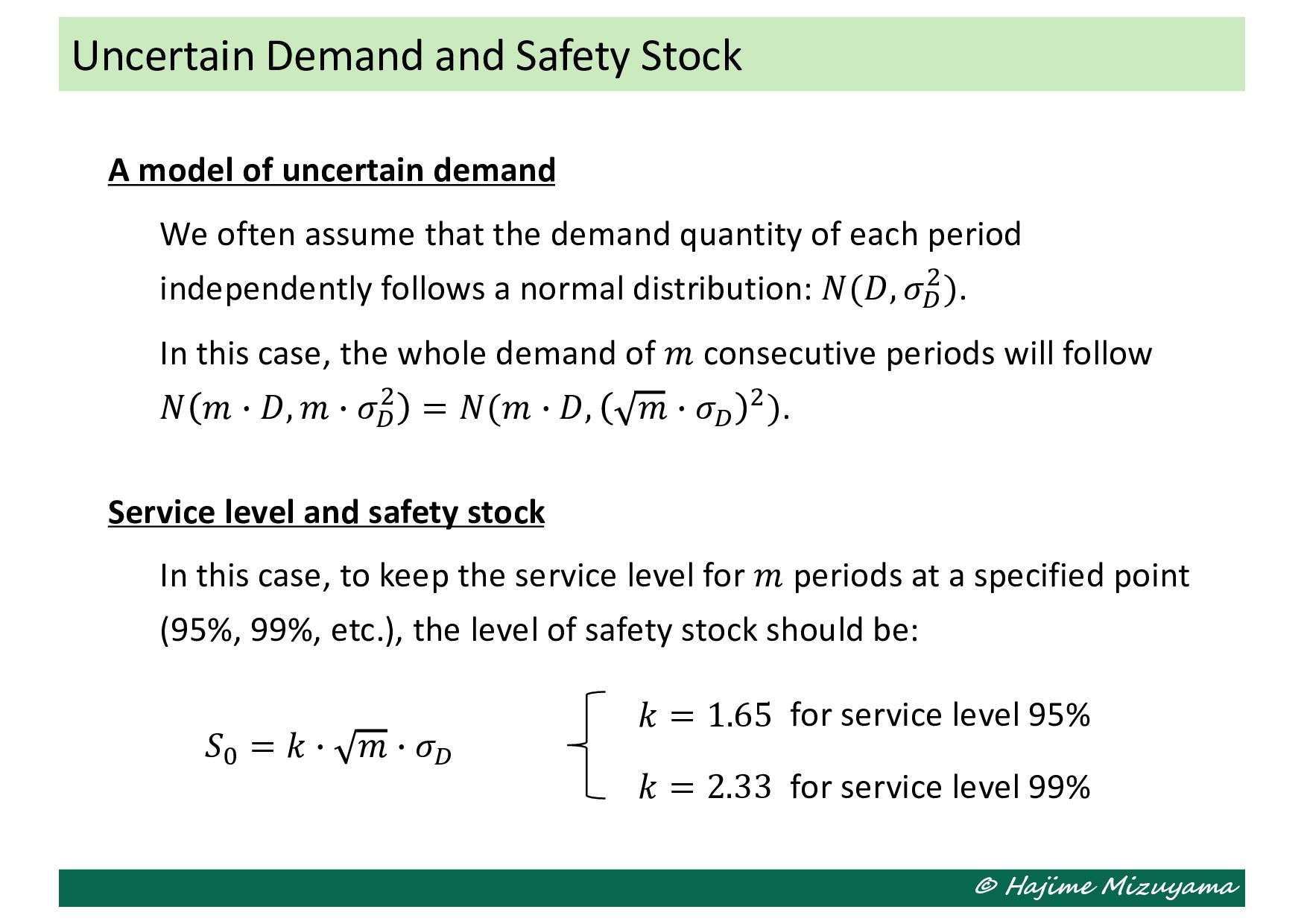
20. © Hajime Mizuyama A model of uncertain demand We often assume that the demand quantity of each period independently follows a normal distribution: 𝑁(𝐷, 𝜎$ %). In this case, the whole demand of 𝑚 consecutive periods will follow 𝑁 𝑚 ) 𝐷, 𝑚 ) 𝜎$ % = 𝑁(𝑚 ) 𝐷, 𝑚 ) 𝜎$ %). Service level and safety stock In this case, to keep the service level for 𝑚 periods at a specified point (95%, 99%, etc.), the level of safety stock should be: Uncertain Demand and Safety Stock 𝑆& = 𝑘 ) 𝑚 ) 𝜎$ 𝑘 = 1.65 𝑘 = 2.33 for service level 95% for service level 99%
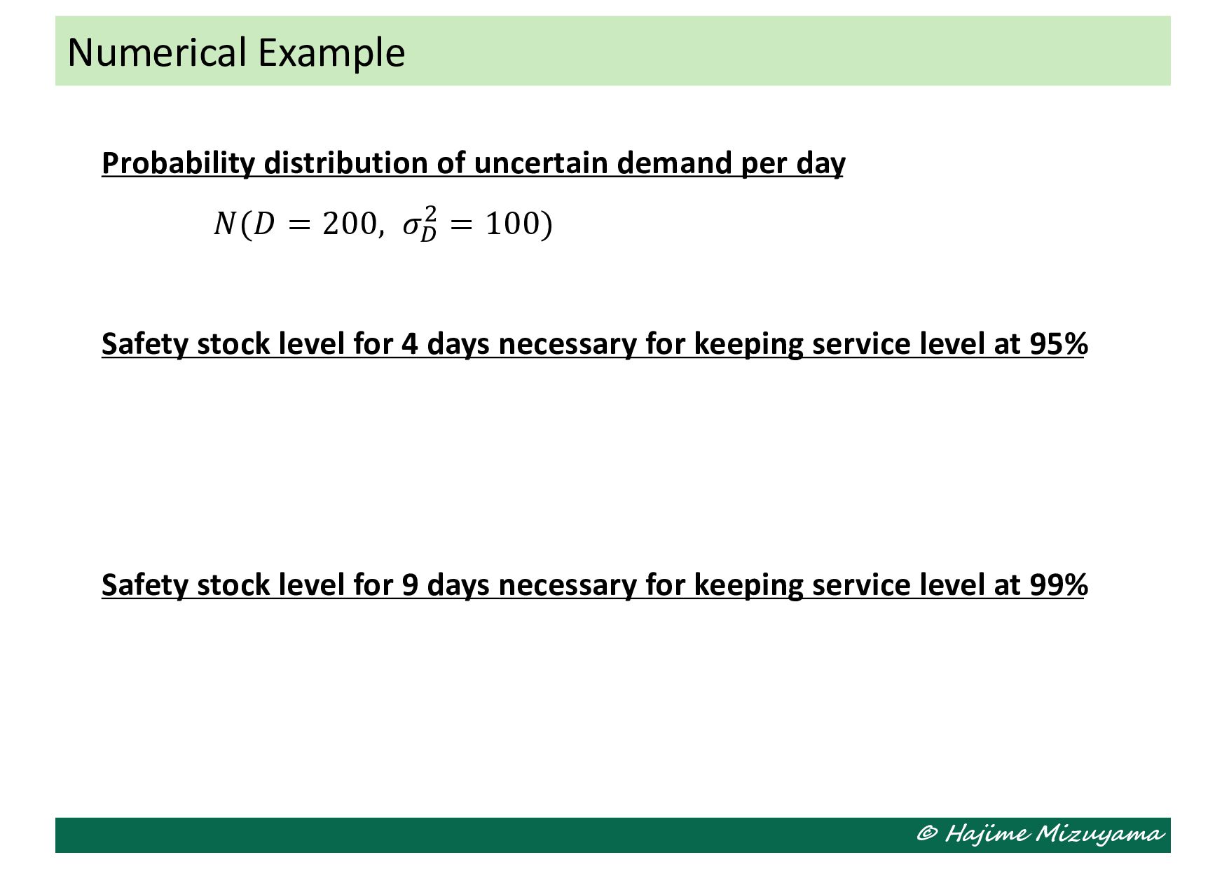
21. © Hajime Mizuyama Probability distribution of uncertain demand per day 𝑁(𝐷 = 200, 𝜎$ % = 100) Safety stock level for 4 days necessary for keeping service level at 95% Safety stock level for 9 days necessary for keeping service level at 99% Numerical Example
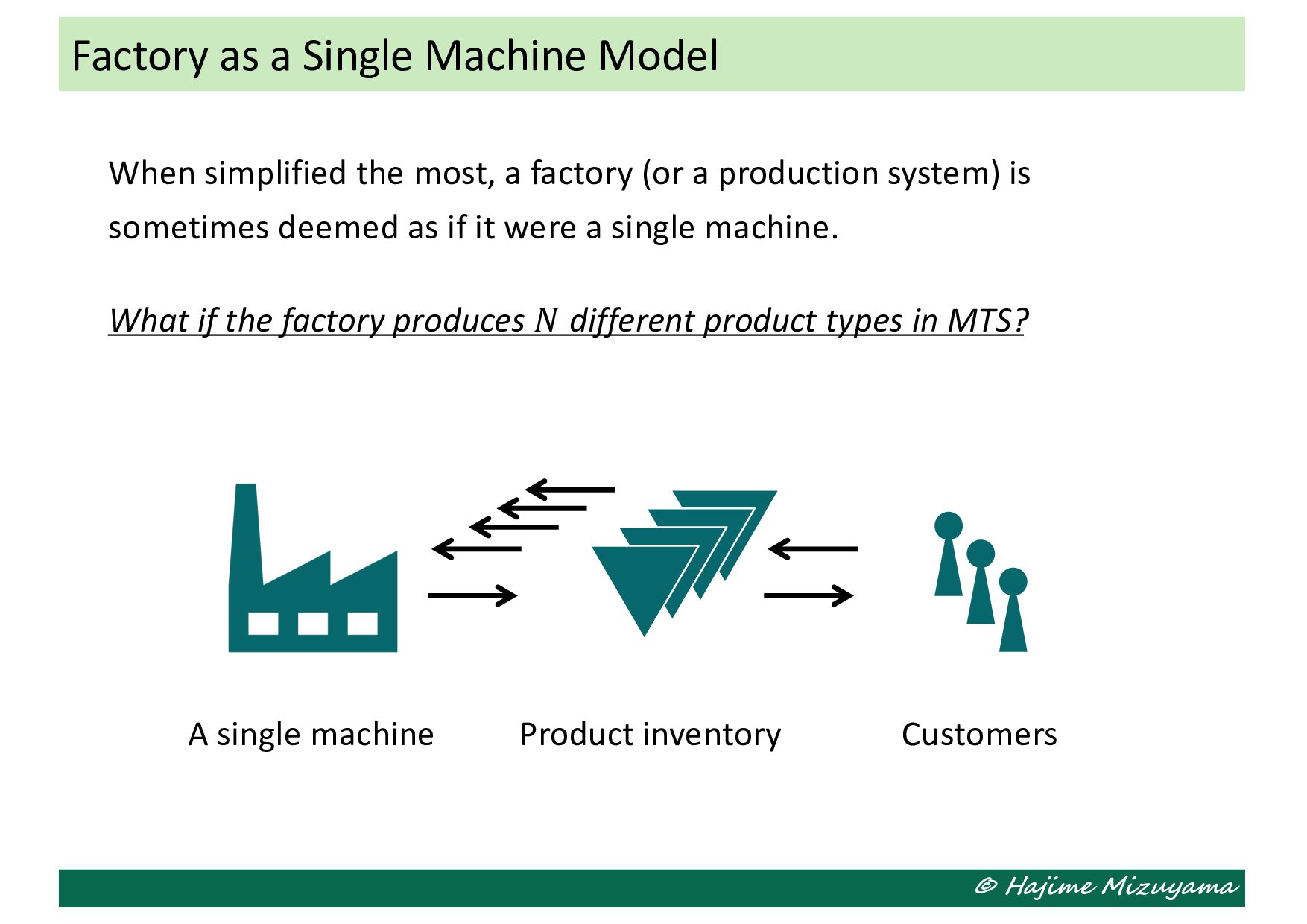
22. © Hajime Mizuyama When simplified the most, a factory (or a production system) is sometimes deemed as if it were a single machine. What if the factory produces 𝑁 different product types in MTS? Factory as a Single Machine Model A single machine Product inventory Customers
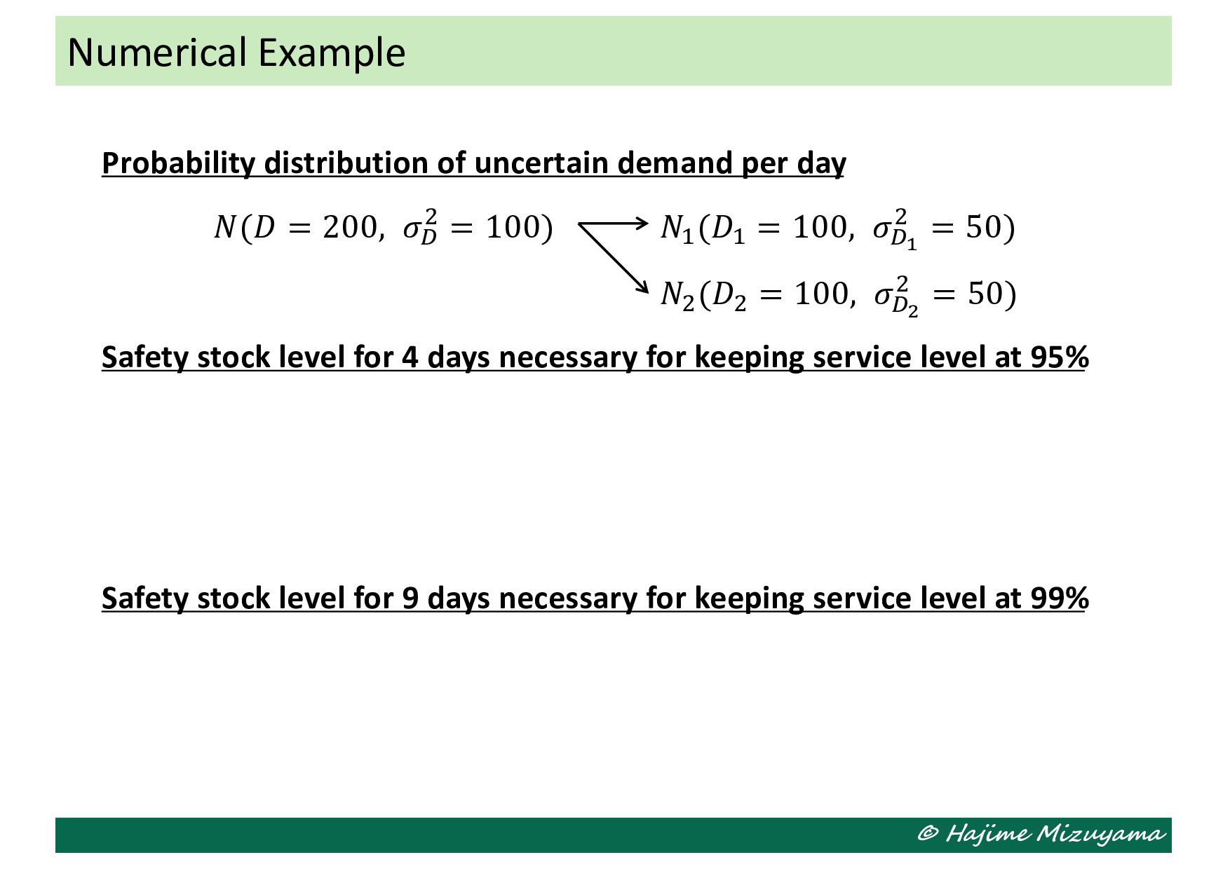
23. © Hajime Mizuyama Probability distribution of uncertain demand per day 𝑁(𝐷 = 200, 𝜎$ % = 100) 𝑁' (𝐷' = 100, 𝜎$! % = 50) 𝑁% (𝐷% = 100, 𝜎$" % = 50) Safety stock level for 4 days necessary for keeping service level at 95% Safety stock level for 9 days necessary for keeping service level at 99% Numerical Example