有關洋流渦輪機的水動力設計 - 辛敬業 副教授

有關洋流渦輪機的水動力設計 - 辛敬業 副教授

Transcript

1. 有關洋流渦輪機的水動力設計 辛敬業1, 王世雲1, 賴信安1, 李綺芳2, 蔡進發3, 邱逢琛3 1國立台灣海洋大學系統工程暨造船學系 2財團法人中國驗船中心 3國立臺灣大學工程科學及海洋工程學系 2019.08.12
2. 1 Kuroshio (黑潮) ▪ High power density / Steady / Persistent ▪ 10(~30)GW : 20% ~ 20億瓦 (200萬瓩 : 核四270萬瓩)
3. 2 FKT Design Requirement ▪ The prototype is 1/5 scale. ▪ The experiment model is 1/25 scale. ▪ Power produced by one turbine need to achieve 10kW. (10kW*2) ▪ 可以調節浮力，利用海流調節 深度，確保機器處於最高效率。 ▪ 受颱風、地震、水災影響小
4. 3 S&T Research Scope ▪ 發展一洋流渦輪機的水動力設計方法 ▪ 應用的方法 ▪ 自升力線方法、升力面方法、邊界元素法(BEM)至 黏性流RANS方法 ▪ 在需要效率的設計問題上，整合不同精確度 (fidelity)的計算方法 ▪ 可以同時滿足時間與精度的要求，達到設計目標 ▪ 計算結果的確認 ▪ Verification: 不同方法 ▪ Validation: 實驗
5. 4 Available Computational Methods ▪ Blade Element Momentum method ▪ Widely used by Wind Turbine Designs and Analysis ▪ Forces ▪ Boundary Element method ▪ Potential Flow ▪ Forces, Pressure Distributions ▪ & Lifting Surface & Lifting Line methods --- Propeller designs ▪ Viscous Flow RANS method ▪ Real Flow ▪ Analysis Design of Blade Geometry  Wind turbine?  Propeller?  Analysis Tools
6. 5 Boundary Element Method ▪ Perturbation potential based ▪ Distributing the dipole and source on the surface panels ▪ Solving for the velocity potentials ▪ Velocity potential -> Velocities -> Pressure -> Forces ▪ Marine propellers --- Current Turbines ▪ Governing equation: ▪ 2 = ׭ [() 1 (:) − 1 : ] + ׭ Δ 1 : ▪ σ =1 , = σ =1 , − σ=1 σ ,. ∆, = 1,
7. 6 Viscous Methods: STAR-CCM+ & SC/Tetra 15R 7.9R 16.1R Velocity Inlet Pressure Outlet Turbine Slip wall Reference Frame-Rotating • Realizable k-ε two-layer models is applied. • Approximately 4 million polyhedral elements 6
8. 7 Foil Geometry NACA66/a=0.8meanline Number of blade 3 Radius(m) 0.4 Rotational Speed(rps) 4.13(Clockwise from inflow) Inflow velocities(m/s) 1.50, 2.00, 2.50, 3.00 Tip Speed Ratio (TSR) 6.92, 5.19, 4.15, 3.46 Analysis Tip Speed Ratio Axial Force coefficient Torque coefficient 2 1 2 Q Q C ARV  = 2 1 2 X X F C AV  = 2 nR TSR V  = 3 2 1 2 W W PW P nQ P C AV   = = Power coefficient
9. 8 Verification: BEM vs. RANS
10. 9 Verification: BEM vs. RANS TSR=5.19 r/R=0.50 r/R=0.90
11. 10 Design of Blade Geometry  Propeller  Potential flow & Viscous Flow methods
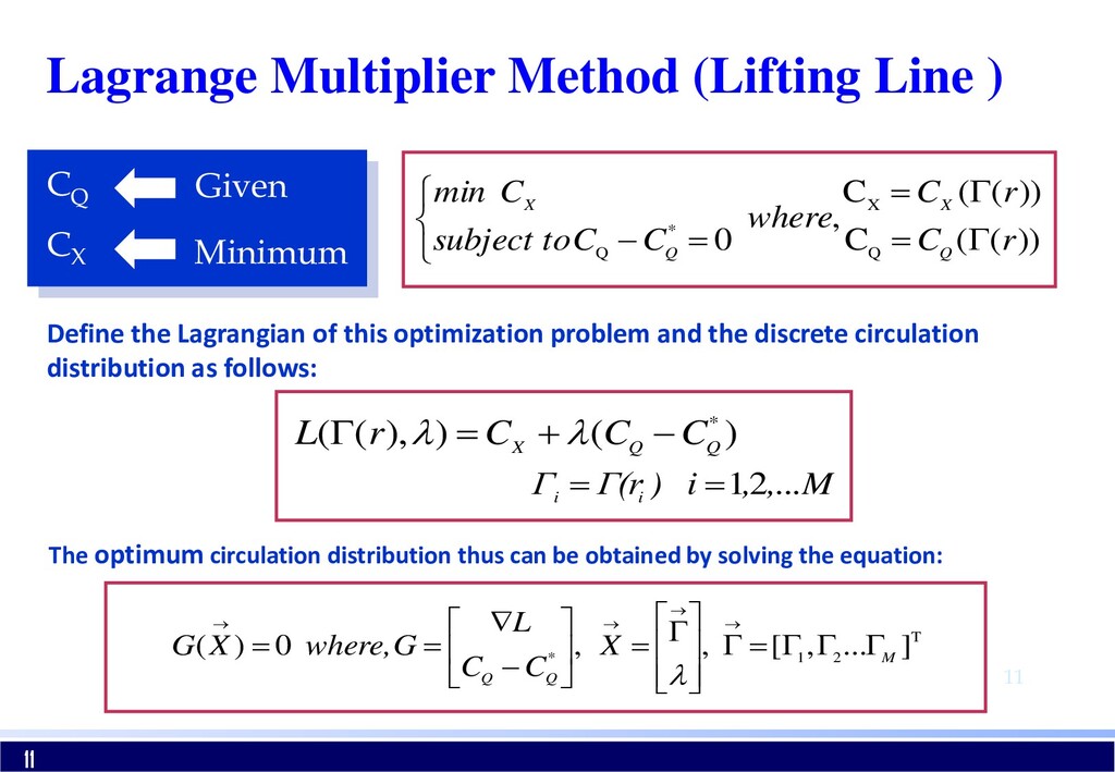
12. 11 Lagrange Multiplier Method (Lifting Line ) CX CQ Minimum Given Define the Lagrangian of this optimization problem and the discrete circulation distribution as follows: ) ( ) ), ( ( * Q Q X C C C r L − + =        =  = = − )) ( ( C )) ( ( C , 0 Q X * Q r C r C where C C subject to C min Q X Q X ] ... , [ , , 0 ) ( T 2 1 * M Q Q X C C L G where, X G    =          =       −  = = → → → →  ,...M , ) i Γ(r Γ i i 2 1 = = The optimum circulation distribution thus can be obtained by solving the equation: 11
13. 12 Axial Force, Torque, Power Pitch (P/D), Camber (f/C) BEM(CTPAN-S) Optimum Circulation Distribution Lifting Surface Theory Lifting Line Theory + Lagrange multiplier method Design Method I.
14. 13 Genetic Algorithm Method Design Complete 13 First generation Objective function Fitness Function Individual A Individual B Next generation Crossover & Mutation Satisfy the objective? No Base Design: Lagrange Multiplier method Max. C Q
15. 14 Design Procedure Lagrange Multiplier method • Potential Flow methods • Design Loading Distributions • Design Blade Geometry: Pitch & Camber Genetic Algorithm • Potential Flow methods: BEM • Improve the Design: Pitch & Camber • Chord-length Designs • …… Analysis & Verification • Potential Flow BEM • Viscous Flow RANS • Verify the Design • Performance Curve
16. 15 Design of the 20kW FKT 1/5 scale, 10kw*2 ◼D=5 m (RH /R=0.24) ◼V=1.5(m/s) ◼rpm=30 1/25 scale, Model Test ◼D=1 m CX CQ CPW BEM 0.70740 0.07905 0.41390 RANS 0.75950 0.08501 0.44510 Fx (N) Q (N-m) Pw (W) BEM 15594.74 4356.67 13686.73 RANS 16743.29 4685.14 14718.44 Fx (N) Q (N-m) Pw (W) BEM 623.79 34.85 547.47 RANS 669.73 37.48 588.74
17. 16 Performance of 3-blade: BEM vs. RANS
18. 17 Performances of different blade numbers Design
19. 18 Performance Curve
20. 19 Validation  Vs. NTU Experiment
21. 20 Compared with Experimental Data ▪ Experiment modal is 1/25 scale. ▪ The experiment was carried out at National Taiwan University towing tank and the measured data were compared with RANS computational result.
22. 21 Compared with Experimental Data ▪ The experimental data (red dot) of thrust coefficient obtained by two turbines rotating clockwise (left figure) and counter clockwise (right figure). ▪ Hydrodynamic performance of a towed floating Kuroshio current turbine Jin-Fa Tsai, Yi-Hsiang Liao, Forng-Chen Chiu, AWTEC2018
23. 22 Compared with Experimental Data ▪ The experimental data (red dot) of torque coefficient obtained by two turbines rotating clockwise (left figure) and counter clockwise (right figure).
24. 23 Compared with Experimental Data ▪ The experimental data (red dot) of power coefficient obtained by two turbines rotating clockwise (left figure) and counter clockwise (right figure).
25. 24 Different Operating Conditions  Overall  One side malfunction  Inclined Inflow  Array
26. 25 Overall FKT Performance Analysis Inflow Velocity (m/s) TSR CT CQ CPW Turbine Only 1.2 5.24 0.7581 0.0807 0.4225 Full FKT (steady) 1.2 5.24 0.7556 0.0804 0.4211 Full FKT (unsteady) 1.2 5.24 0.7658 0.0807 0.4224 ▪ It is obvious that whether there is a floating body or not, the differences are not large.
27. 26 Overall FKT Performance Analysis ▪ The magnitude of force variation on each blade is about 2% (left figure). ▪ Total force on one turbine, the force fluctuation is only 0.6% (right figure). 2% 0.6%
28. 27 Simulation of One Side Malfunction TURBINE 1 2 Inflow velocity (m/s) 1.5 1.5 Rotational speed (rps) 0.5 0 malfunction Turbine 1 Turbine 2 Axial Force (N) 16819.12 Axial Force (N) 4315.63 Torque (N-m) 4548.61 Torque (N-m) 1271.32
29. 28 Top View
30. 29 Inclined Inflow
31. 30 FKT Array ▪ Body Force method
32. 31 Conclusions ▪ Design Procedure of FKT & Validation ▪ Hydrodynamic Design: BEM & RANS ▪ Lagrange Multiplier method ▪ Genetic Algorithm ▪ Computational results are compared with experimental data and achieve the design goal ▪ Simulations of different possible operating conditions ▪ A practical and reliable current turbine design procedure
33. 32 Thank You for listening hsin@mail.ntou.edu.tw