Masters Defense Presentation

9/2/2014 Masters Defense at University of Tokyo IST Computer Science

Transcript

1. A Parallel Greedy Hill-climbing Algorithm for Bayesian Network Estimation Matthew Barga Suda Laboratory 9/2/2014
2. Introduction to Bayesian Networks • Represents a set of random variables and their dependencies • Constructed as a Directed Acyclic Graph (DAG) • Visual output provides an intuitive tool to understand causal relationships in data History of Smoking Tumor in lung Cancer Chronic Bronchitis DAG of a Bayesian network showing the causalities among features in a medical diagnosis. Vertices represent the random variables and directed edges encode the conditional probabilities.
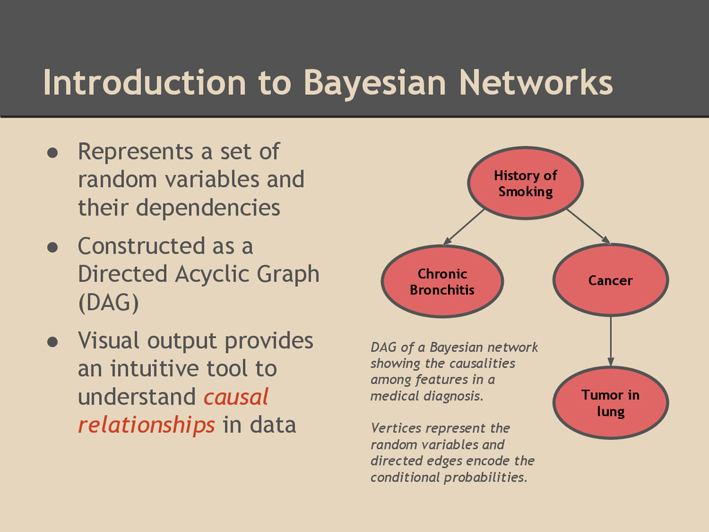
3. Introduction to Bayesian Networks • Structurally represents the joint probability of a set of random variables • Markov assumption: all variables in the network are independent of their non-descendants given their descendants • The set of all direct ascendants of a vertex is referred to as the parent set X 2 X 3 X 4 X 5 X 1 P(X 1 ,X 2 ,X 3 ,X 4 ,X 5 ) = P(X 1 )P(X 2 )P(X 3 |X 1 ,X 4 )P(X 4 |X 2 )P(X 5 |X 3 ,X 4 ) Parent set of X 5 : PaG(X 5 ) = {X 3 ,X 4 } Joint probability of graph G above:
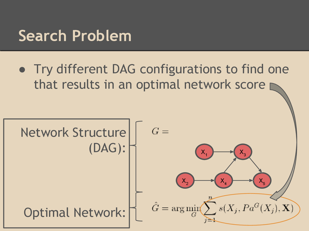
4. Estimation • Algorithms are used to estimate Bayesian networks from data • Search and Score methods are a common approach ◦ Scoring function used to assign a quantitative value to the optimality of an estimated network ◦ Search function used to find network structures that achieve better scores
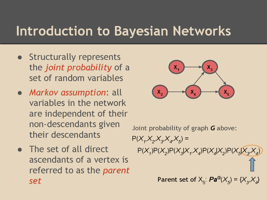
5. Recall Joint Probability Function • Joint probability function decomposes into the product of individual variable density functions conditioned on their parent sets • Simplifies computation by allowing local conditional probabilities to be calculated independently for each variable
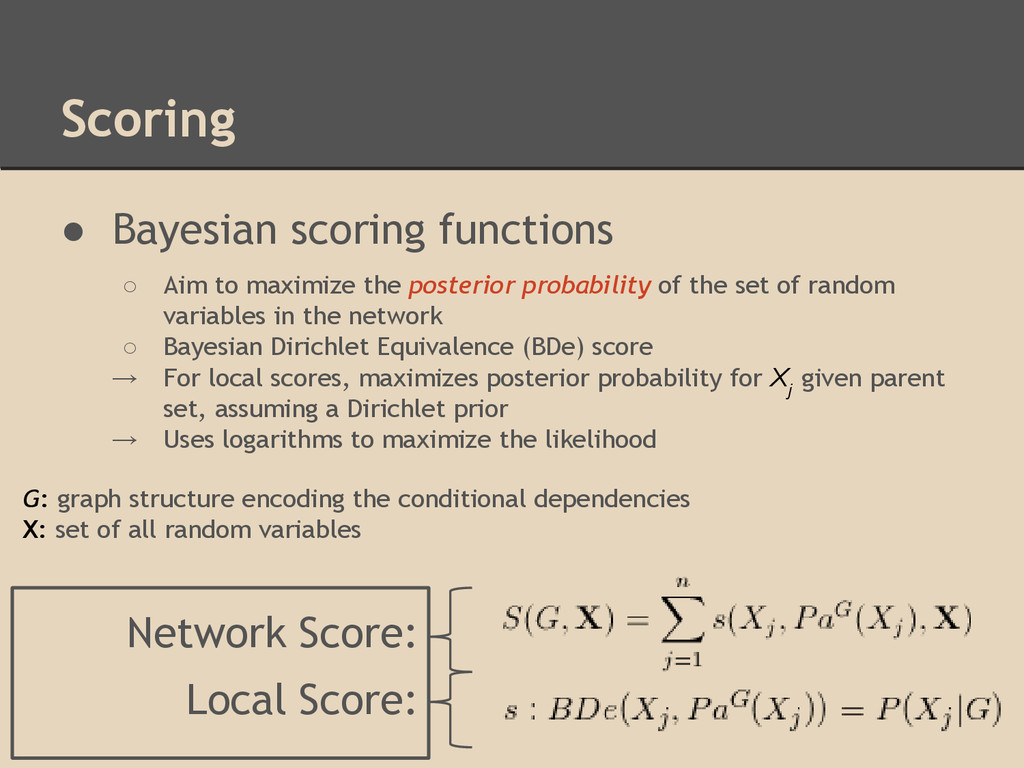
6. • Bayesian scoring functions ◦ Aim to maximize the posterior probability of the set of random variables in the network ◦ Bayesian Dirichlet Equivalence (BDe) score → For local scores, maximizes posterior probability for X j given parent set, assuming a Dirichlet prior → Uses logarithms to maximize the likelihood Scoring Network Score: Local Score: G: graph structure encoding the conditional dependencies X: set of all random variables
7. Search Problem Network Structure (DAG): Optimal Network: X 1 X 2 X 3 X 4 X 5 • Try different DAG configurations to find one that results in an optimal network score
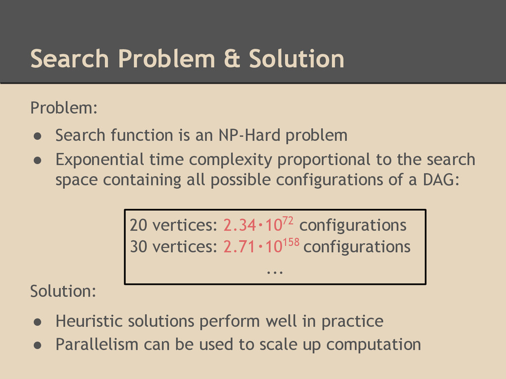
8. Search Problem & Solution Problem: • Search function is an NP-Hard problem • Exponential time complexity proportional to the search space containing all possible configurations of a DAG: Solution: • Heuristic solutions perform well in practice • Parallelism can be used to scale up computation 20 vertices: 2.34・1072 configurations 30 vertices: 2.71・10158 configurations ...
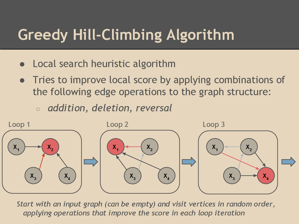
9. Greedy Hill-Climbing Algorithm • Local search heuristic algorithm • Tries to improve local score by applying combinations of the following edge operations to the graph structure: ◦ addition, deletion, reversal X 1 X 4 X 1 X 3 X 3 X 2 X 4 X 2 X 3 X 1 X 4 X 2 Loop 1 Loop 2 Loop 3 Start with an input graph (can be empty) and visit vertices in random order, applying operations that improve the score in each loop iteration
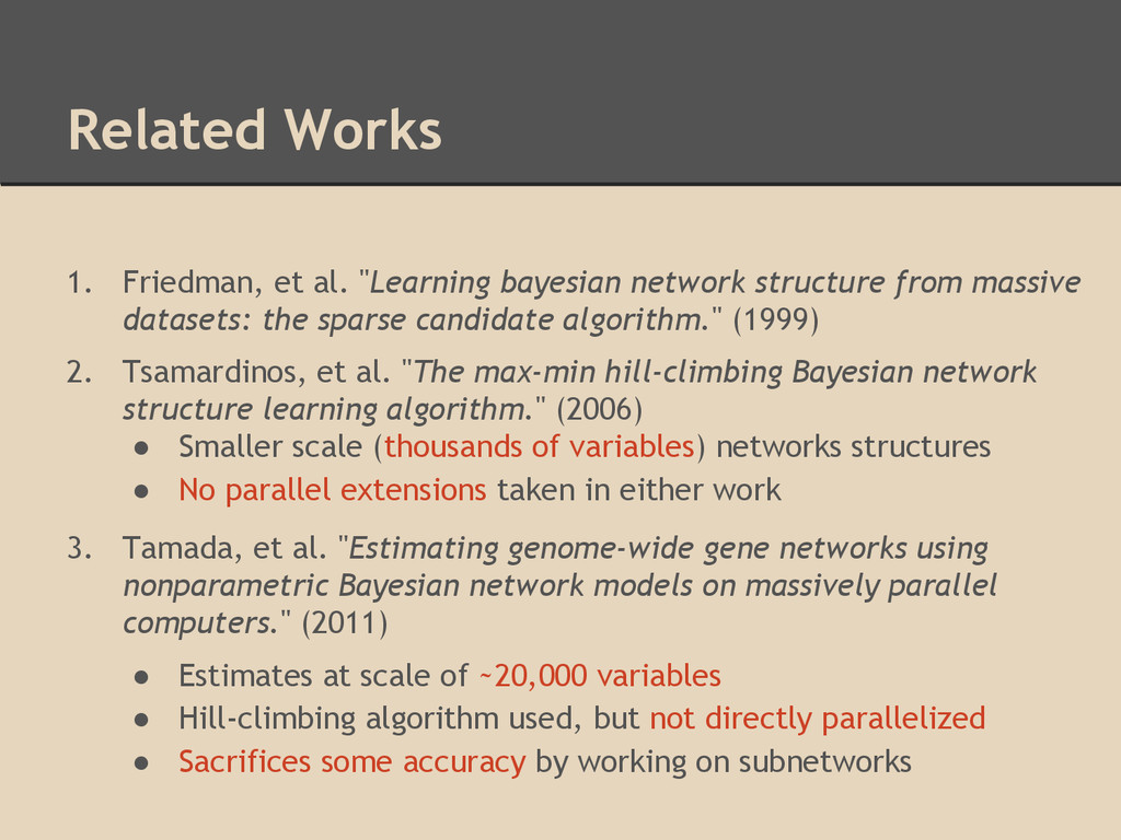
10. Related Works 1. Friedman, et al. "Learning bayesian network structure from massive datasets: the sparse candidate algorithm." (1999) 2. Tsamardinos, et al. "The max-min hill-climbing Bayesian network structure learning algorithm." (2006) • Smaller scale (thousands of variables) networks structures • No parallel extensions taken in either work 3. Tamada, et al. "Estimating genome-wide gene networks using nonparametric Bayesian network models on massively parallel computers." (2011) • Estimates at scale of ~20,000 variables • Hill-climbing algorithm used, but not directly parallelized • Sacrifices some accuracy by working on subnetworks
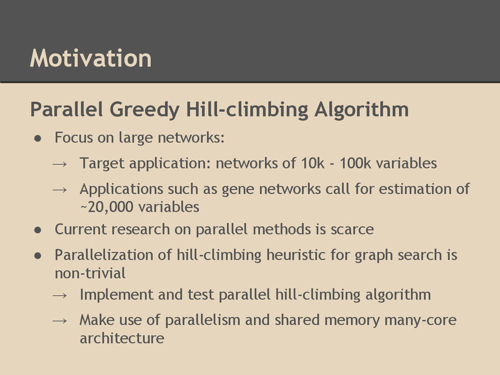
11. Motivation Parallel Greedy Hill-climbing Algorithm • Focus on large networks: → Target application: networks of 10k - 100k variables → Applications such as gene networks call for estimation of ~20,000 variables • Current research on parallel methods is scarce • Parallelization of hill-climbing heuristic for graph search is non-trivial → Implement and test parallel hill-climbing algorithm → Make use of parallelism and shared memory many-core architecture
12. Parallel Greedy Hill-Climbing T1, T2 and T3 represent separate threads. Each thread tries to improve the local scores of the red vertices simultaneously. T1 T2 T3 Repeat until no improvement Output Network
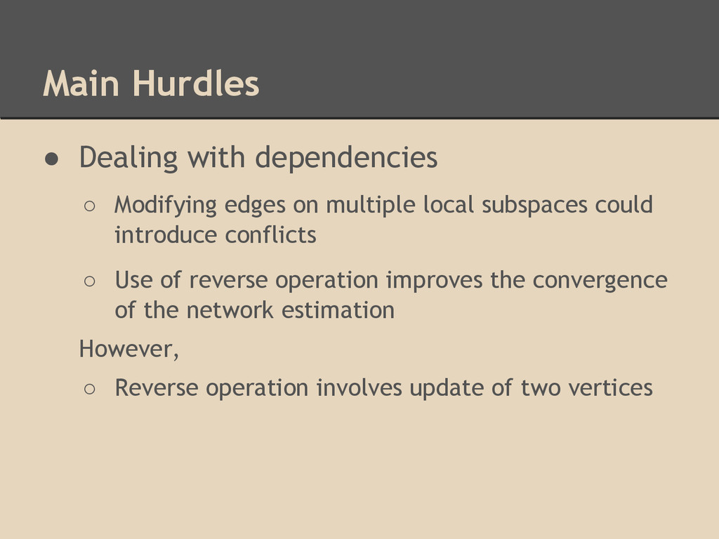
13. Main Hurdles • Dealing with dependencies ◦ Modifying edges on multiple local subspaces could introduce conflicts ◦ Use of reverse operation improves the convergence of the network estimation However, ◦ Reverse operation involves update of two vertices
14. Solution • Collect all operations to be applied to the graph rather than immediately applying them • Process each operation sequentially and look for conflicts among the set of operations
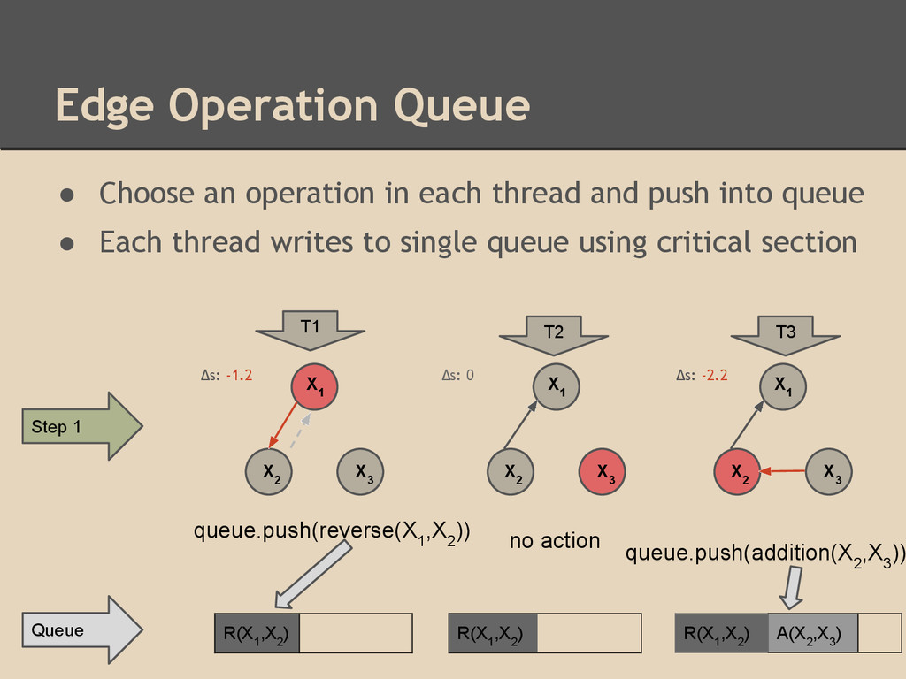
15. Edge Operation Queue • Choose an operation in each thread and push into queue • Each thread writes to single queue using critical section T1 T2 T3 Δs: 0 Δs: -2.2 Δs: -1.2 Step 1 X 1 X 2 X 3 X 3 X 1 X 2 X 3 X 1 X 2 queue.push(reverse(X 1 ,X 2 )) no action queue.push(addition(X 2 ,X 3 )) R(X 1 ,X 2 ) R(X 1 ,X 2 ) R(X 1 ,X 2 ) A(X 2 ,X 3 ) Queue
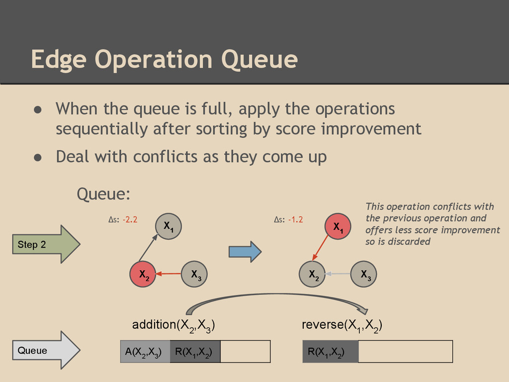
16. Edge Operation Queue • When the queue is full, apply the operations sequentially after sorting by score improvement • Deal with conflicts as they come up Δs: -2.2 Δs: -1.2 Step 2 X 3 X 1 X 2 X 3 X 1 X 2 reverse(X 1 ,X 2 ) addition(X 2 ,X 3 ) Queue: This operation conflicts with the previous operation and offers less score improvement so is discarded A(X 2 ,X 3 ) R(X 1 ,X 2 ) R(X 1 ,X 2 ) Queue
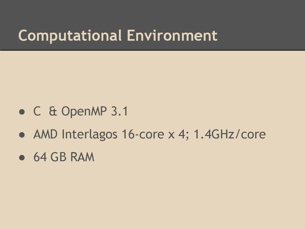
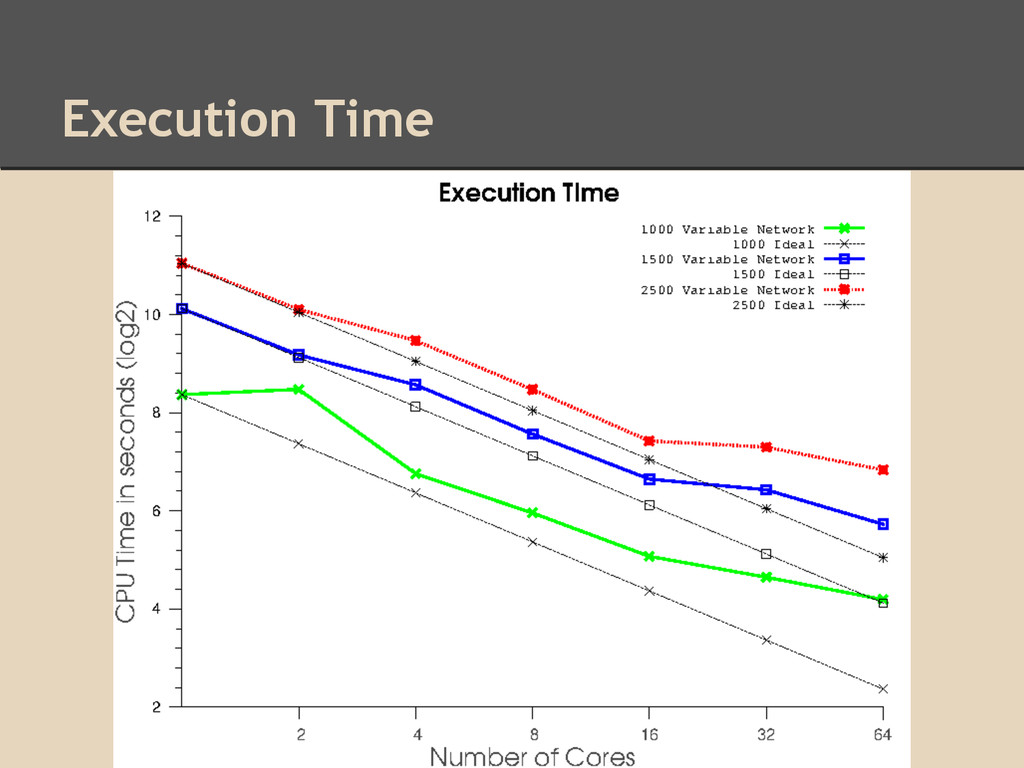
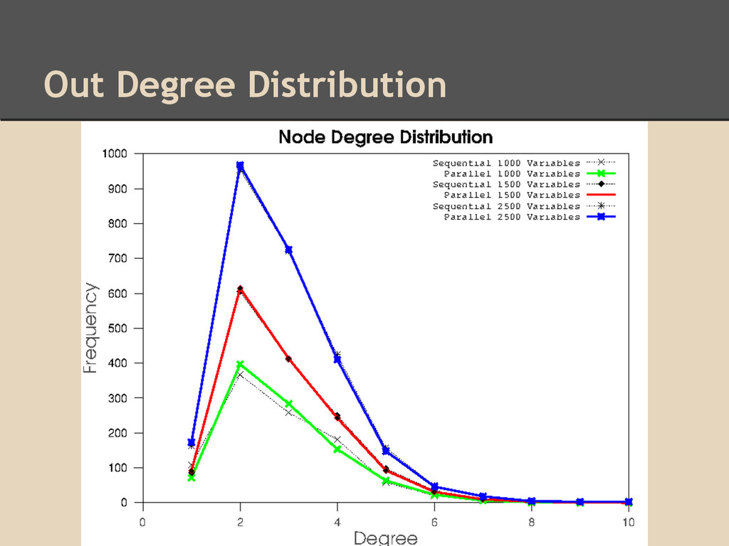
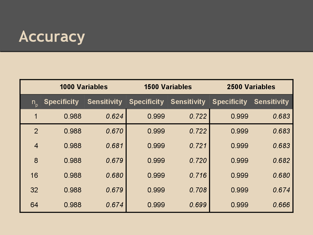
17. Simulation Study 1. The following slides present the results of 3 separate experiments: ◦ 1000 random variables with 1000 samples/variable ◦ 1500 random variables with 1500 samples/variable ◦ 2500 random variables with 1000 samples/variable Goals: 1. Analyze parallel scalability 2. Ensure that accuracy is not sacrificed in parallel algorithm by comparing the parallel hill-climbing algorithm to the sequential version
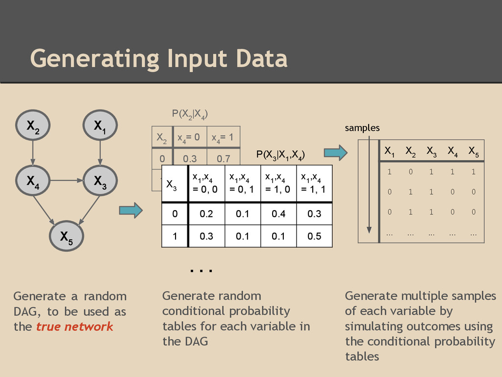
18. Generating Input Data Generate a random DAG, to be used as the true network X 1 X 2 X 3 X 4 X 5 X 2 x 4 = 0 x 4 = 1 0 0.3 0.7 1 0.1 0.9 X 3 x 1 ,x 4 = 0, 0 x 1 ,x 4 = 0, 1 x 1 ,x 4 = 1, 0 x 1 ,x 4 = 1, 1 0 0.2 0.1 0.4 0.3 1 0.3 0.1 0.1 0.5 . . . P(X 2 |X 4 ) P(X 3 |X 1 ,X 4 ) X 1 X 2 X 3 X 4 X 5 1 0 1 1 1 0 1 1 0 0 0 1 1 0 0 ... ... ... ... ... Generate random conditional probability tables for each variable in the DAG Generate multiple samples of each variable by simulating outcomes using the conditional probability tables samples
19. Computational Environment • C & OpenMP 3.1 • AMD Interlagos 16-core x 4; 1.4GHz/core • 64 GB RAM
20. Execution Time
21. Execution Time Breakdown HC . . . HC Initialization and Finalization 3% Queue Flush 2% HC [95%] -> calc_score ~99% 64-Thread Parallel Hill-Climbing: • Variance among individual thread times in HC < 4 sec.
22. Parallel Scaling
23. Accuracy • Out degree for vertices should remain similar between sequential and parallel implementations • Edges in estimated networks should match corresponding edges in true network (sensitivity and specificity)
24. Out Degree Distribution
25. Accuracy 1000 Variables 1500 Variables 2500 Variables n p Specificity Sensitivity Specificity Sensitivity Specificity Sensitivity 1 0.988 0.624 0.999 0.722 0.999 0.683 2 0.988 0.670 0.999 0.722 0.999 0.683 4 0.988 0.681 0.999 0.721 0.999 0.683 8 0.988 0.679 0.999 0.720 0.999 0.682 16 0.988 0.680 0.999 0.716 0.999 0.680 32 0.988 0.679 0.999 0.708 0.999 0.674 64 0.988 0.674 0.999 0.699 0.999 0.666
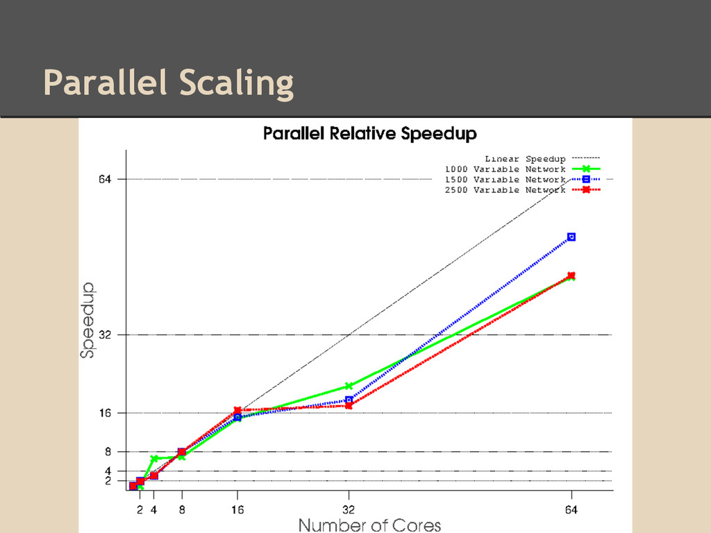
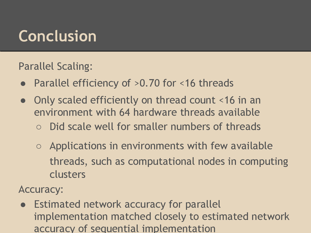
26. Conclusion Parallel Scaling: • Parallel efficiency of >0.70 for <16 threads • Only scaled efficiently on thread count <16 in an environment with 64 hardware threads available ◦ Did scale well for smaller numbers of threads ◦ Applications in environments with few available threads, such as computational nodes in computing clusters Accuracy: • Estimated network accuracy for parallel implementation matched closely to estimated network accuracy of sequential implementation
27. END