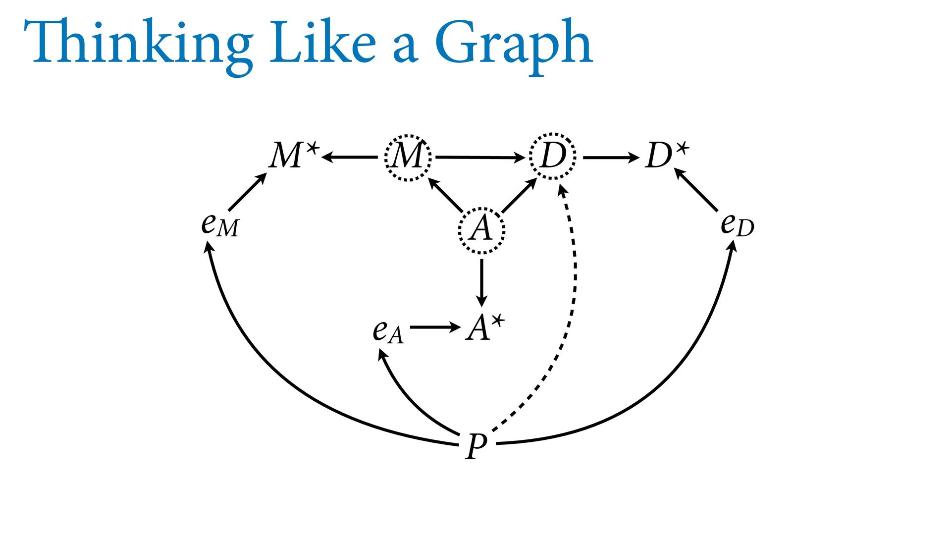
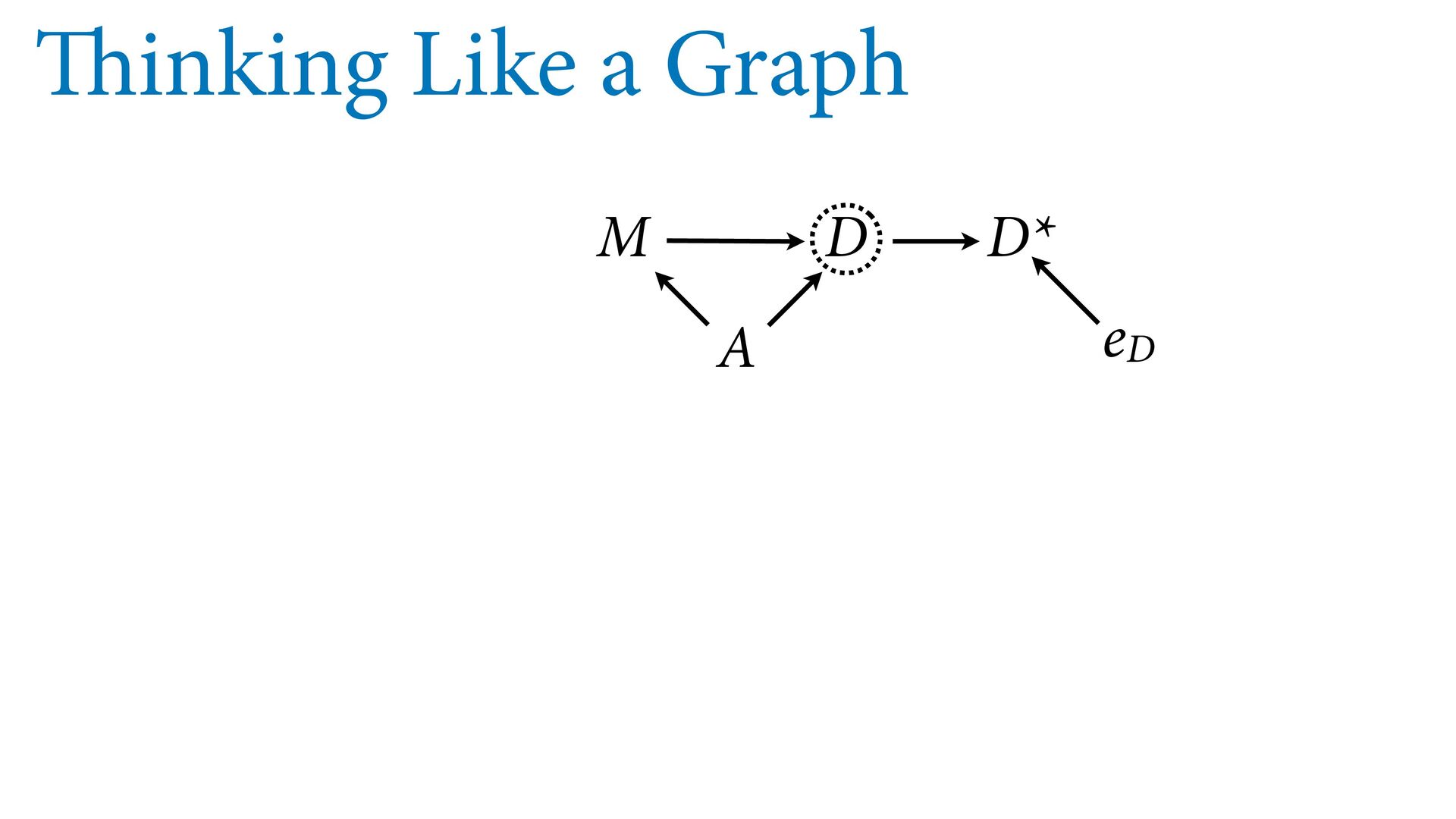
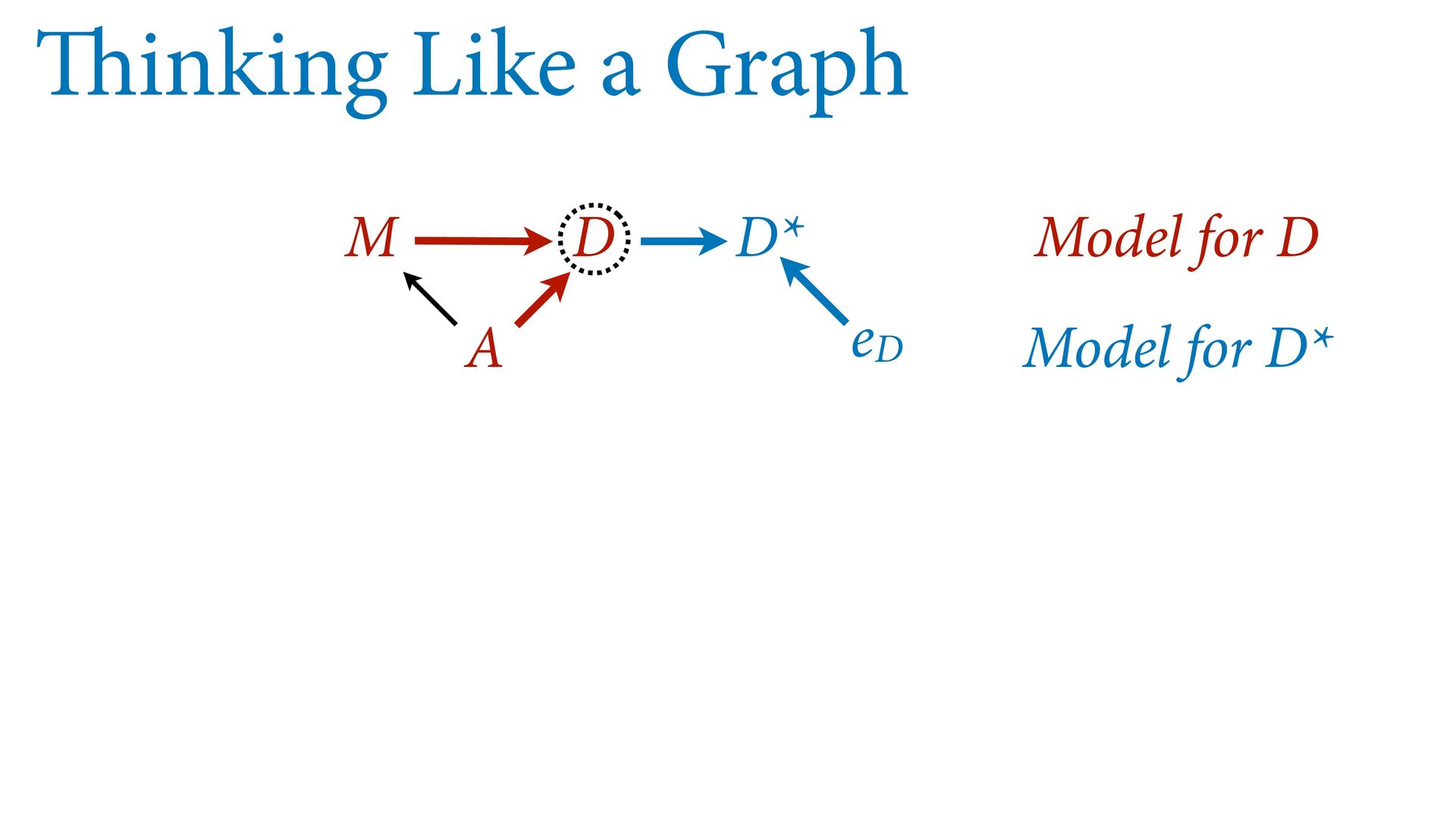
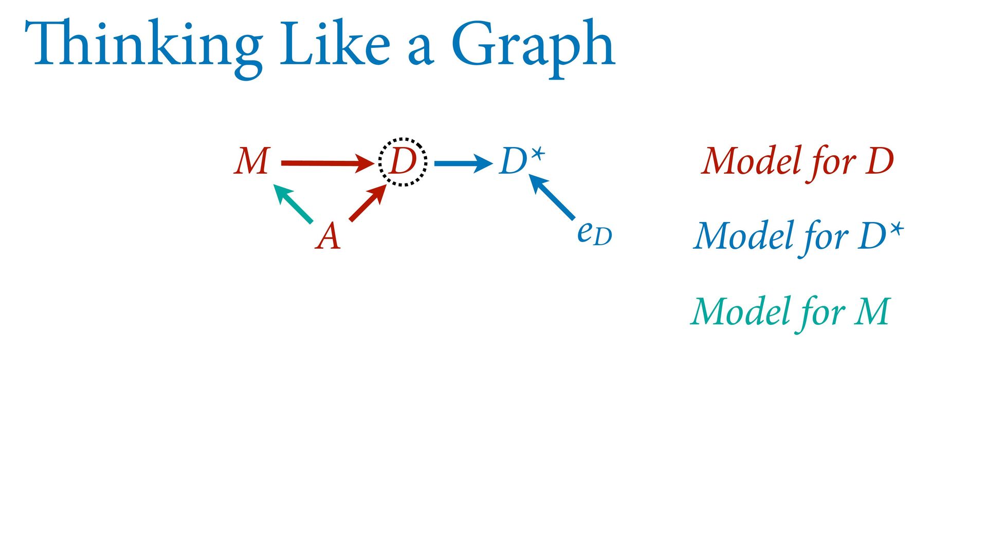
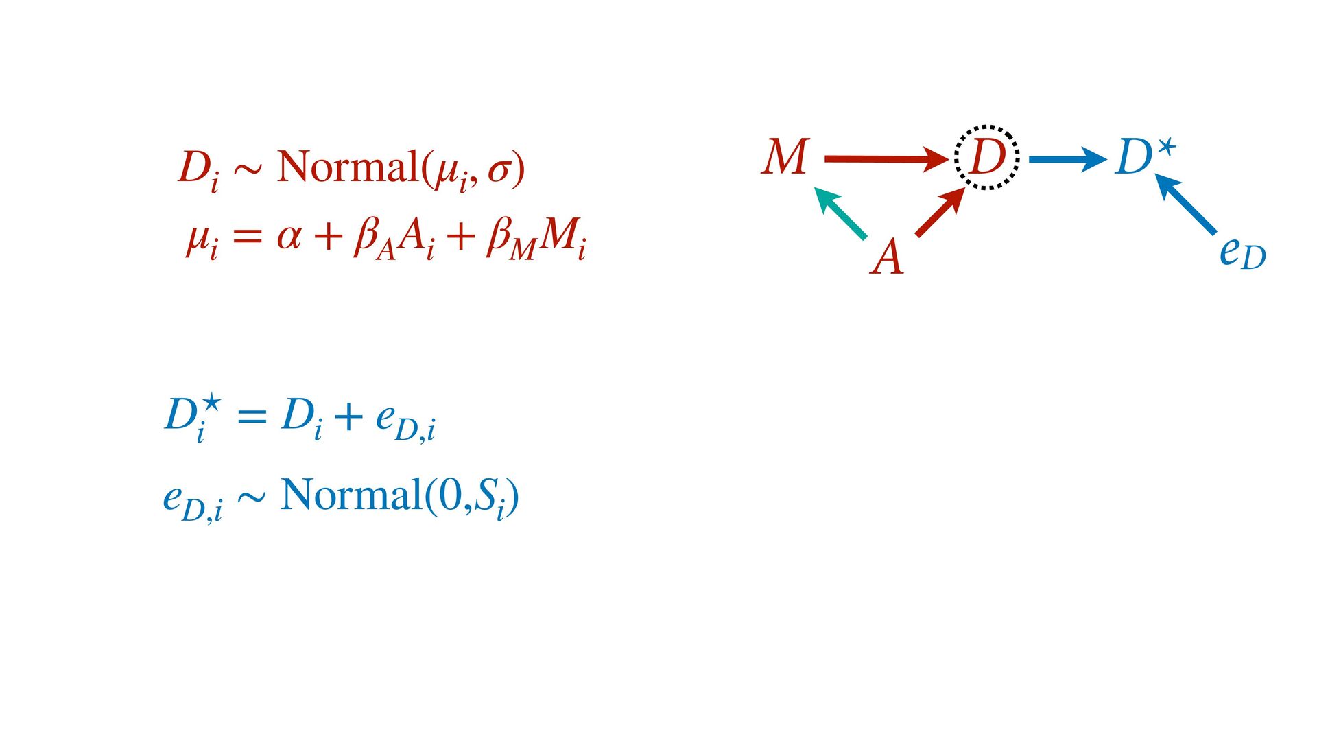
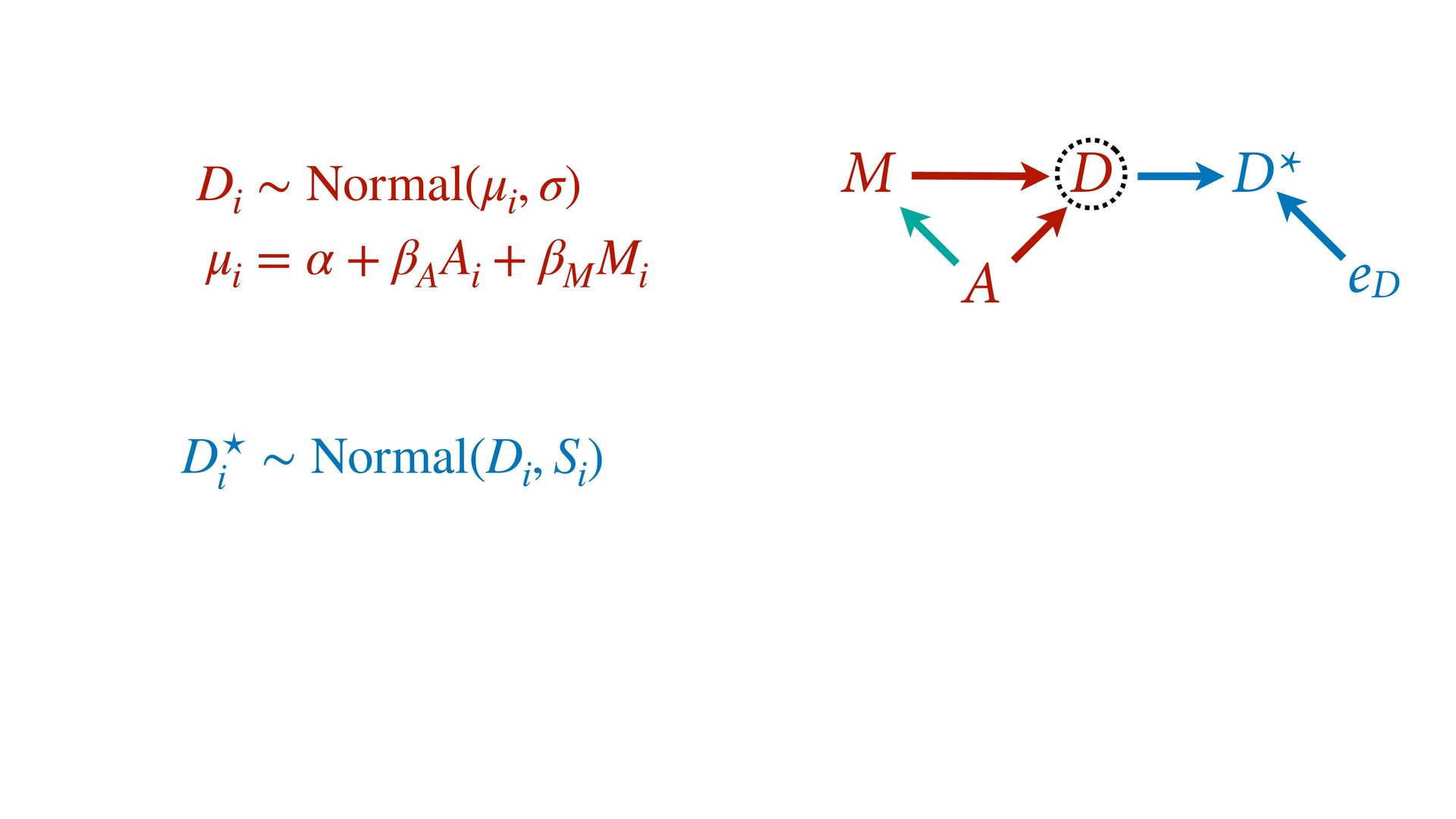
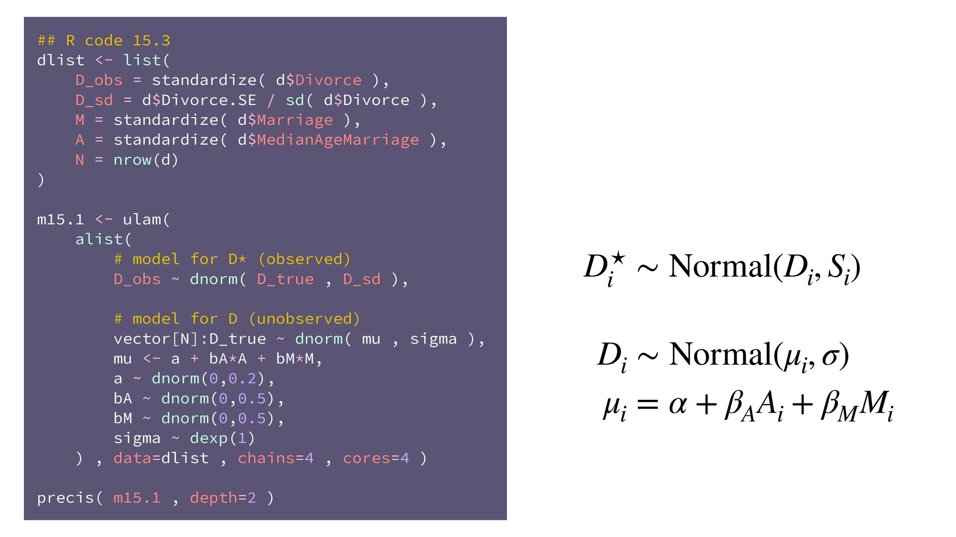
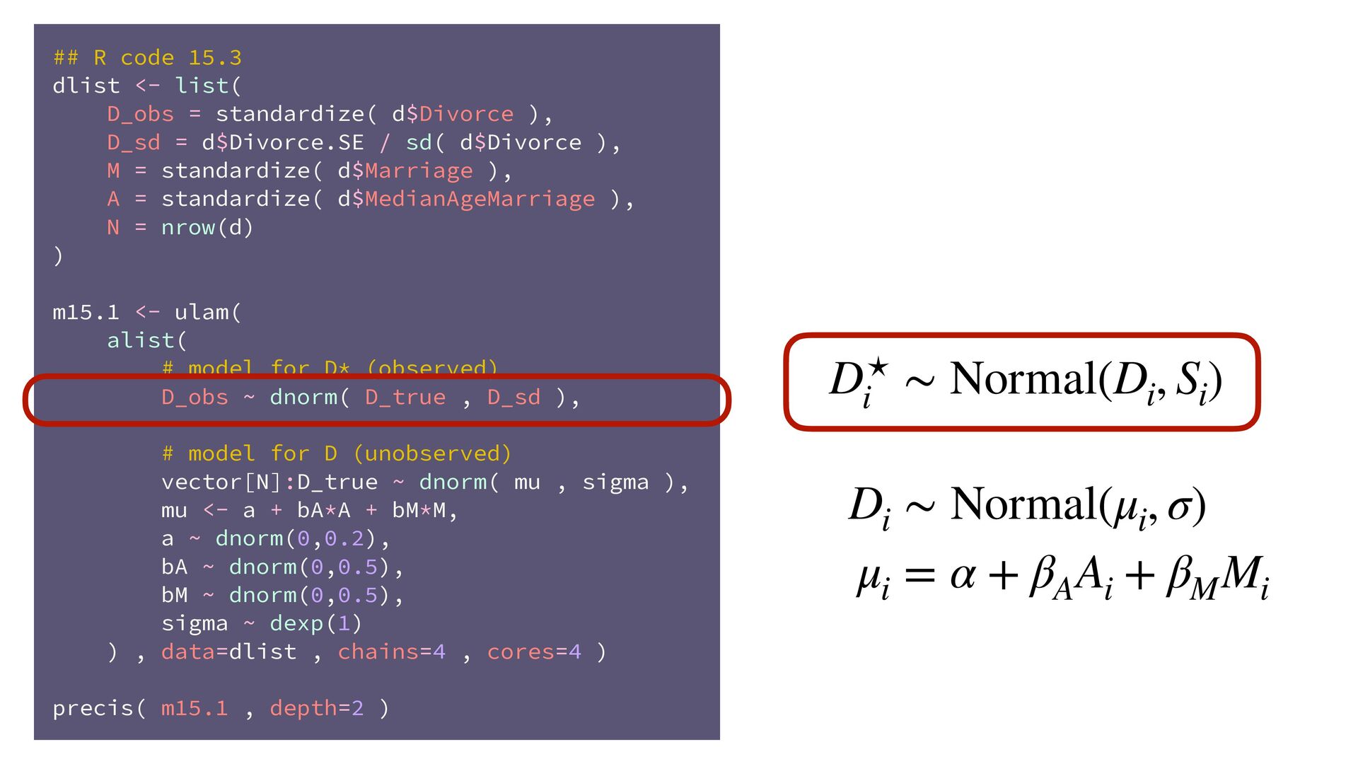
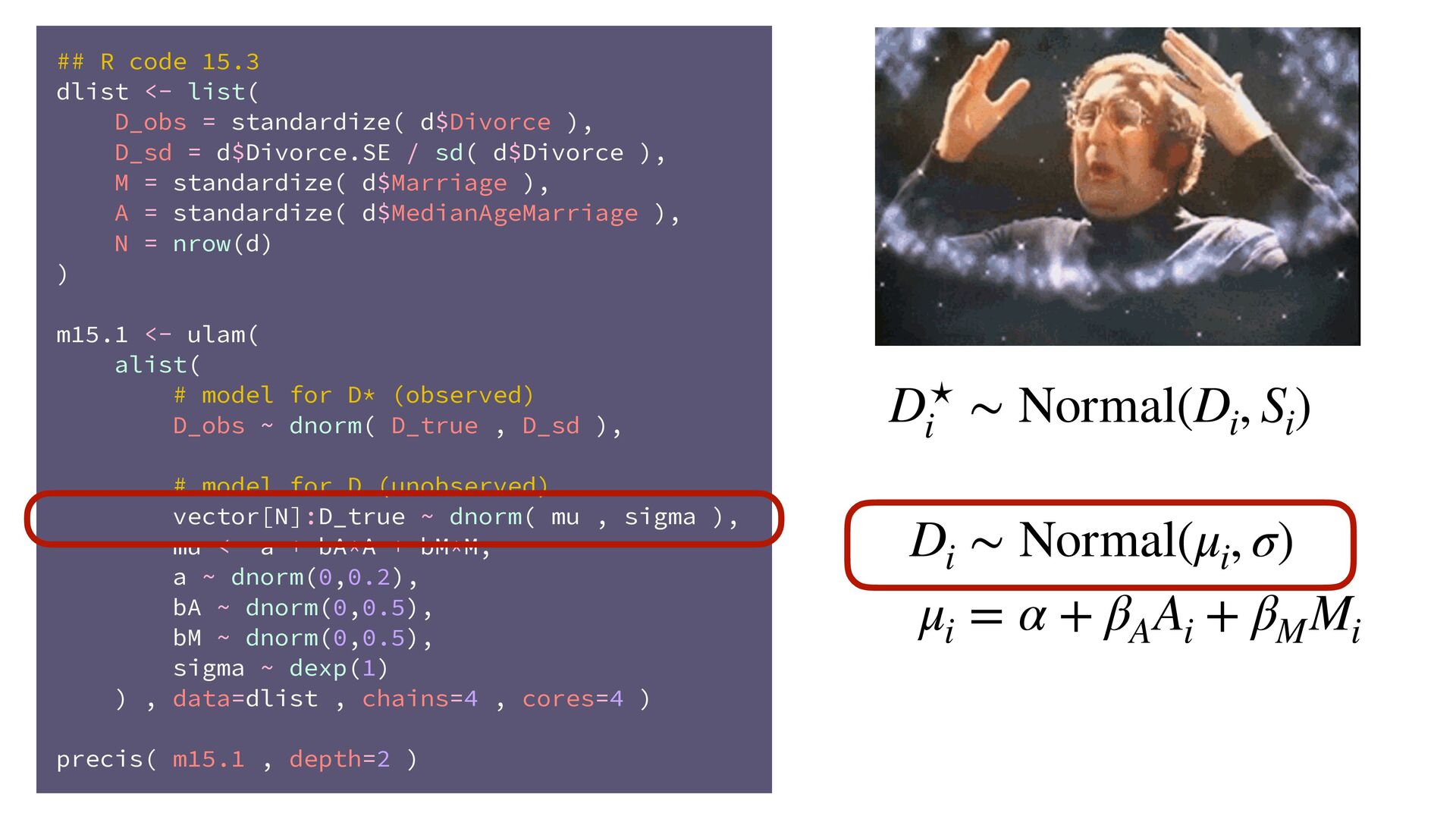
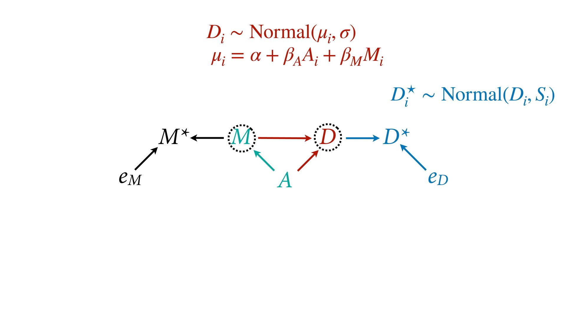
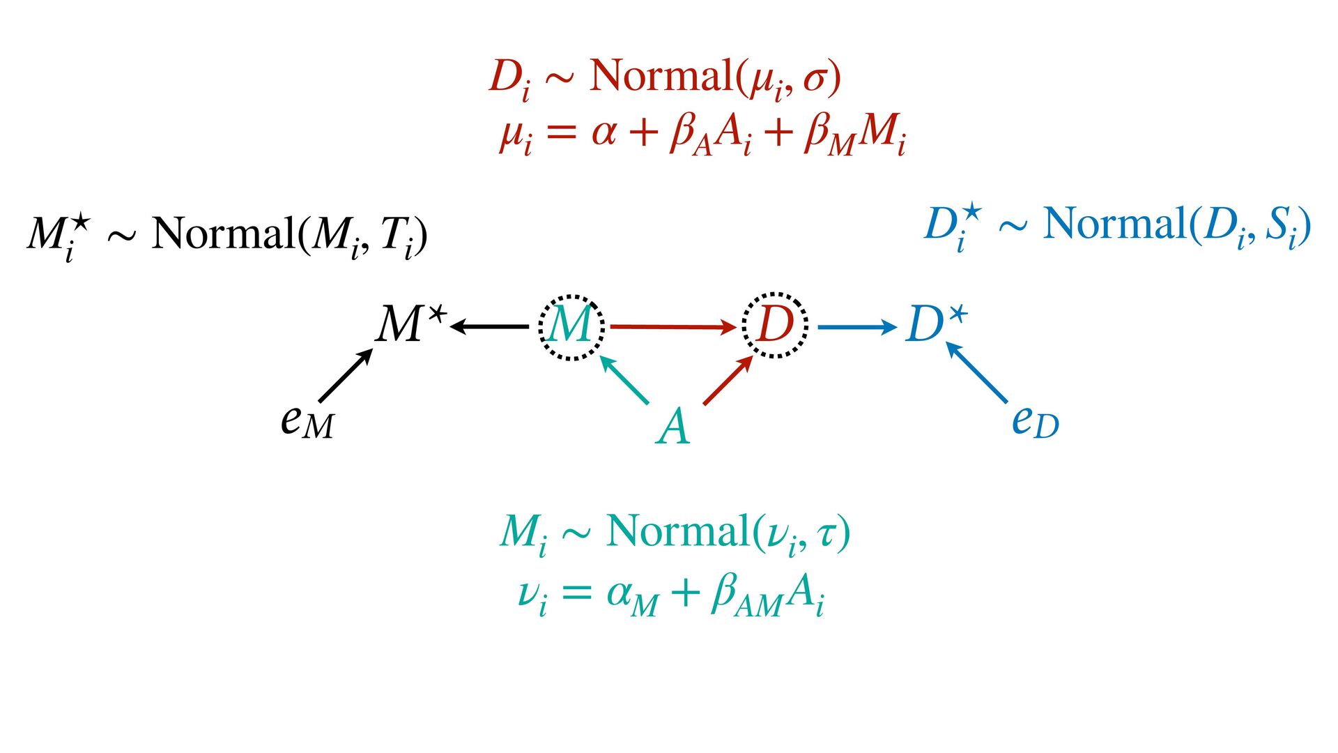
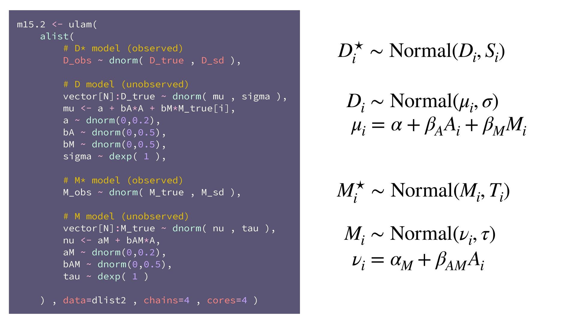
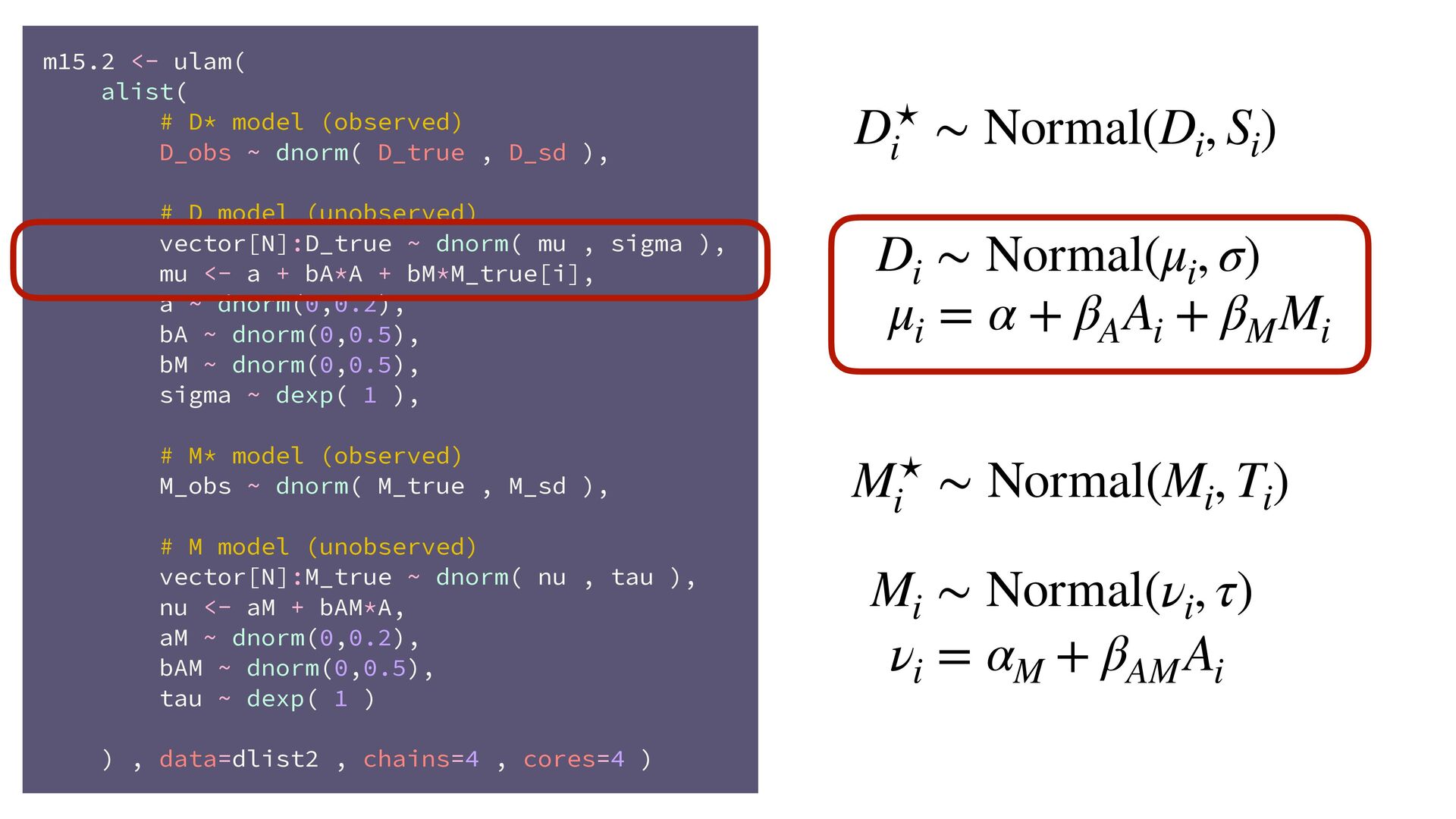
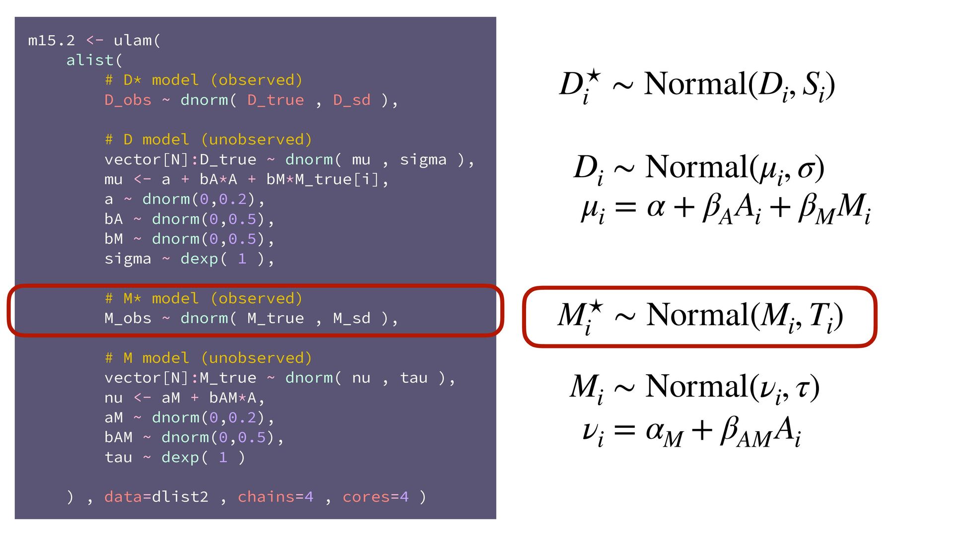
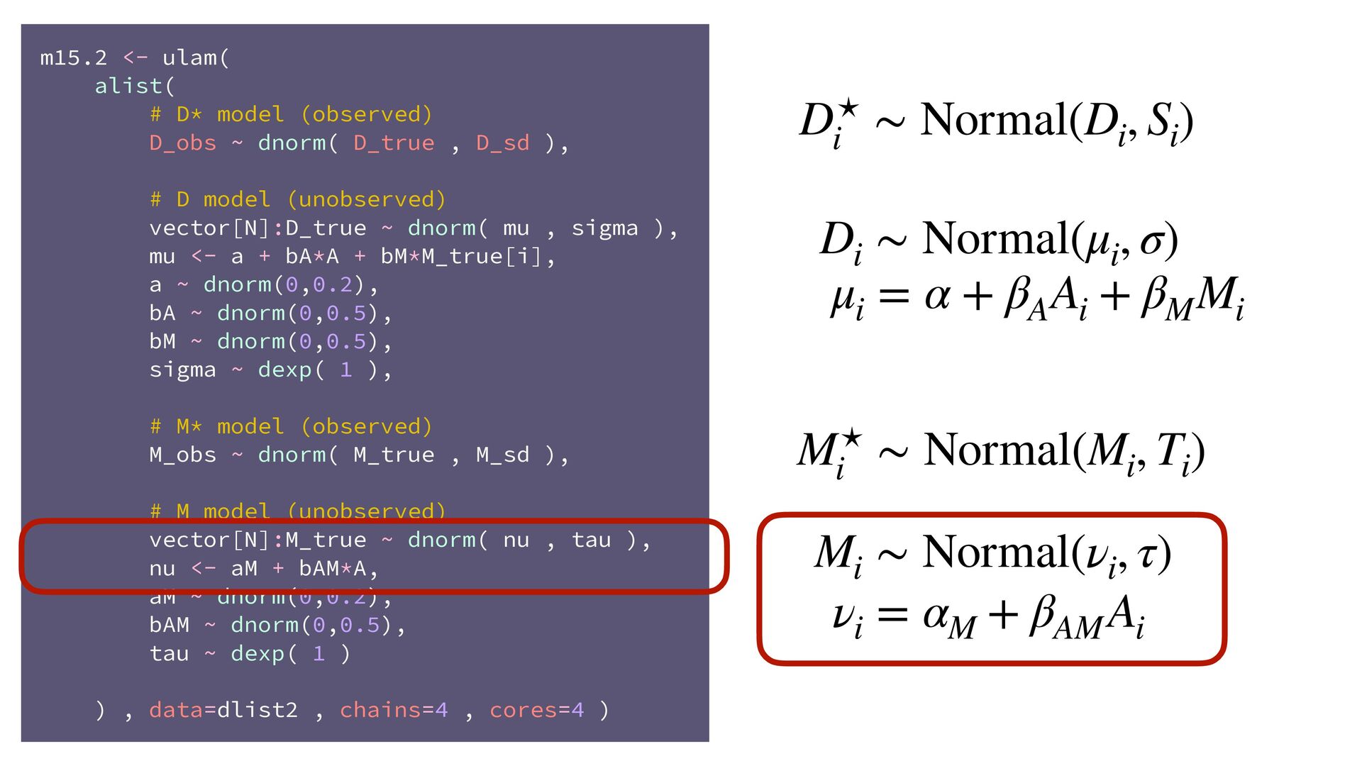
dnorm( D_true , D_sd ), # D model (unobserved) vector[N]:D_true ~ dnorm( mu , sigma ), mu <- a + bA*A + bM*M_true[i], a ~ dnorm(0,0.2), bA ~ dnorm(0,0.5), bM ~ dnorm(0,0.5), sigma ~ dexp( 1 ), # M* model (observed) M_obs ~ dnorm( M_true , M_sd ), # M model (unobserved) vector[N]:M_true ~ dnorm( nu , tau ), nu <- aM + bAM*A, aM ~ dnorm(0,0.2), bAM ~ dnorm(0,0.5), tau ~ dexp( 1 ) ) , data=dlist2 , chains=4 , cores=4 ) M⋆ i ∼ Normal(M i , T i ) D⋆ i ∼ Normal(D i , S i ) M i ∼ Normal(ν i , τ) ν i = α M + β AM A i D i ∼ Normal(μ i , σ) μ i = α + β A A i + β M M i