Masters thesis defense talk

High dimensional Gaussian processes.

Transcript

1. GAUSSIAN PROCESSES WITH BUILT-IN DIMENSIONALITY REDUCTION SCHOOL OF MECHANICAL ENGINEERING PURDUE UNIVERSITY APPLICATIONS IN HIGH-DIMENSIONAL UNCERTAINTY PROPAGATION 1 ROHIT TRIPATHY MAJOR PROFESSOR: PROF. ILIAS BILIONIS COMMITTEE MEMBERS: PROF. ALINA ALEXEENKO PROF. MARISOL KOSLOWSKI IN COLLABORATION WITH: PROF. MARCIAL GONZALEZ.
2. UNCERTAINTY QUANTIFICATION 2 • quantitative characterization and reduction of uncertainties. • Objectively assess confidence in a given prediction. • Effect of limited knowledge in inputs.
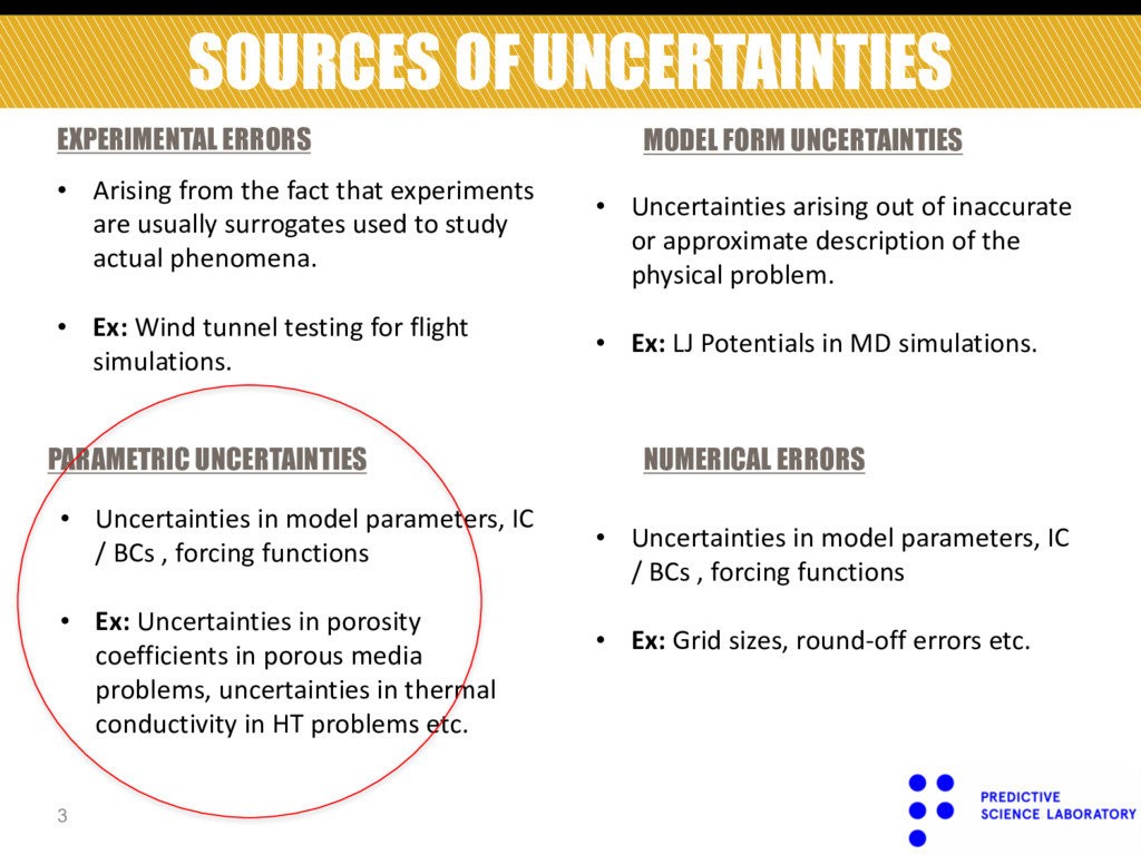
3. SOURCES OF UNCERTAINTIES 3 EXPERIMENTAL ERRORS • Arising from the fact that experiments are usually surrogates used to study actual phenomena. • Ex: Wind tunnel testing for flight simulations. MODEL FORM UNCERTAINTIES • Uncertainties arising out of inaccurate or approximate description of the physical problem. • Ex: LJ Potentials in MD simulations. PARAMETRIC UNCERTAINTIES • Uncertainties in model parameters, IC / BCs , forcing functions • Ex: Uncertainties in porosity coefficients in porous media problems, uncertainties in thermal conductivity in HT problems etc. NUMERICAL ERRORS • Uncertainties in model parameters, IC / BCs , forcing functions • Ex: Grid sizes, round-off errors etc.
4. UNCERTAINTY PROPAGATION PROBLEM • Given the map : • Formally: • Output statistics: x → y = f (x) p(x) → p(y) = δ ∫ (y − f (x))p(x)dx 4 µ f = f ∫ (x)p(x)dx σ f 2 = ( f ( ∫ x)− µ f )2 p(x)dx
5. MONTE CARLO 5 • Simplest way to propagate uncertainty. • Convergence rate independent of number of dimensions. • “Monte Carlo is Fundamentally Unsound”, O’Hagan (1987). Error~O 1 N ⎛ ⎝ ⎜ ⎞ ⎠ ⎟
6. SURROGATE MODELS 6 • expensive computer code à cheap-to-evaluate surrogate. • Examples: § generalized polynomial chaos § Radial basis functions (RBF) § Gaussian Process Regression (GPR) § …. CURSE OF DIMENSIONALITY !!
7. THE CURSE OF DIMENSIONALITY 7
8. DEALING WITH HIGH-DIMENSIONS Generic, long-term, approach: • Exploit invariances, special structure. • non-linear manifolds. Here, we focus on: • HD input. • linear manifold. 8
9. ACTIVE SUBSPACE METHODOLOGIES Input: x Output: y ! !f :!D → !,D ≫1 Reduced input: z ! ! !z = Wx ∈!d ,d ≪ D ! !g:!d → ! Orthogonal projection matrix Gaussian process regression 9
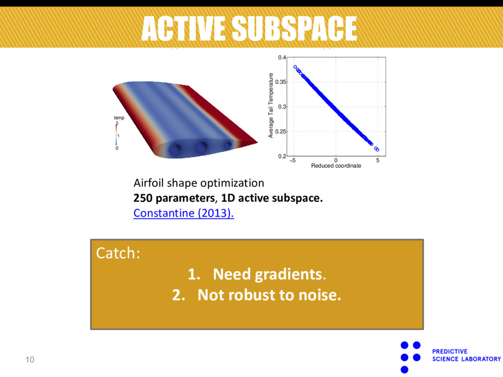
10. ACTIVE SUBSPACE (a) 0 2 1 temp (b) −5 0 5 0.2 0.25 0.3 0.35 0.4 Reduced coordinate Average Tail Temperature Figure 2: We examined a model for heat transfer in a turbine blade given a parameterized model for the heat flux boundary condition representing unknown transition to turbulence. There are 250 parameters characterizing a Karhunen-Loeve model of the heat flux, and the quantity of interest is the average tem- perature over the trailing edge of the blade. The leftmost figure shows the domain and a representative temperature distribution. The rightmost figure plots 750 samples of the quantity of interest against the projected coordinate. The strong appearance of the linear relationship verifies the quality of the subspace approximation. (a) (b) 2.55 2.6 2.65 e [bar] Airfoil shape optimization 250 parameters, 1D active subspace. Constantine (2013). Catch: 1. Need gradients. 2. Not robust to noise. 10
11. CLASSIC ACTIVE SUBSPACE REGRESSION • Approximate: • Eigen-decomposition: C = E ∇ x f (x)∇ x f (x)T ⎡ ⎣ ⎤ ⎦ = ∫∇ x f (x)∇ x f (x)T p(x)dx. C = WΛWT C = E ∇ x f (x)∇ x f (x)T ⎡ ⎣ ⎤ ⎦ ≈ 1 N ∇ x i=1 N ∑ f x(i) ( )∇ x f x(i) ( )T 11
12. ACTIVE SUBSPACE METHODOLOGIES Input: x Output: y ! !f :!D → !,D ≫1 Reduced input: z ! ! !z = Wx ∈!d ,d ≪ D Orthogonal projection matrix Gaussian process regression 12 ! !g:!d → !
13. • GP à generalization of a multivariate normal distribution to infinite dimensions. GAUSSIAN PROCESS REGRESSION D projected = z(i) = Wx(i),y(i) = f (x(i) ) ( ) { } i=1 N ! !g:!d → ! ! ! g(⋅)~GP g(⋅)|m(⋅),k 0 (⋅,⋅) ( ). mean function covariance function 13
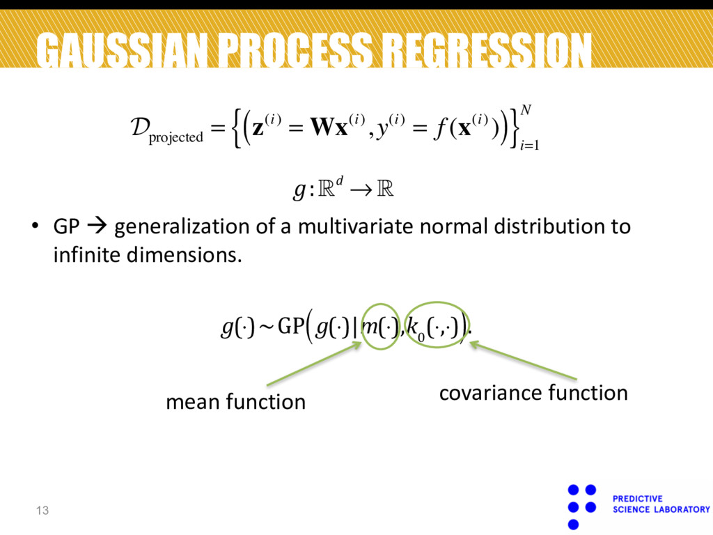
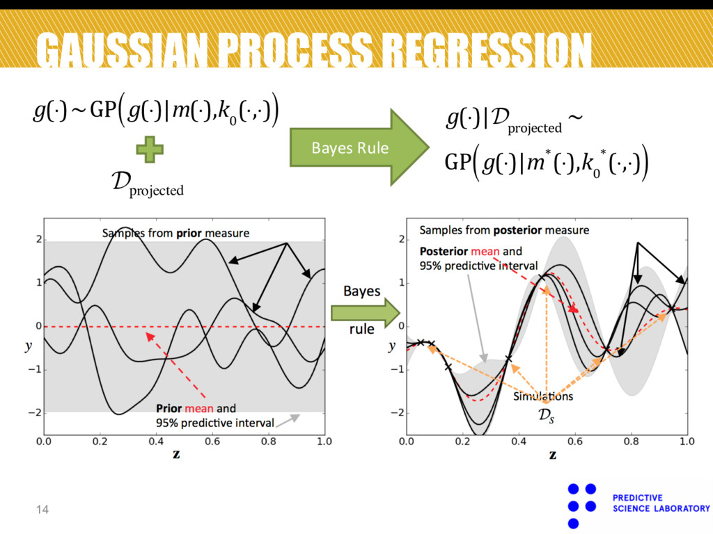
14. GAUSSIAN PROCESS REGRESSION ! ! g(⋅)~GP g(⋅)|m(⋅),k 0 (⋅,⋅) ( ) D projected Bayes Rule ! ! g(⋅)|D projected ~ GP g(⋅)|m*(⋅),k 0 *(⋅,⋅) ( ) Figure 6 - Prior (a) and posterior (b) on the space of 1D functions using Gaussian processes. The red dashed-line indicates the mean of the prior (a) and posterior (b) probability measures. The grey shaded area indicates 95% predictive intervals within which the true law is believed to be. The solid black lines are functional samples from th prior (a) and posterior (b) probability measures. The ‘x’ symbols in (b) indicate simulations, !!, on which we condition 14
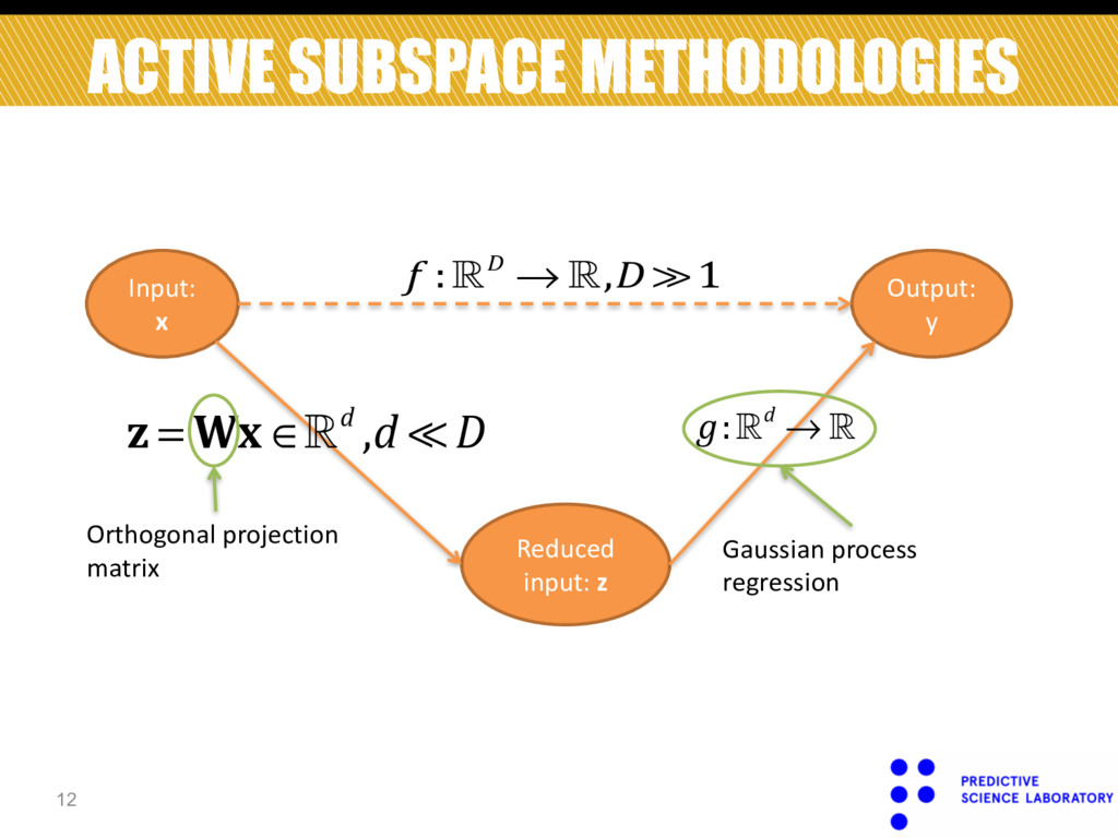
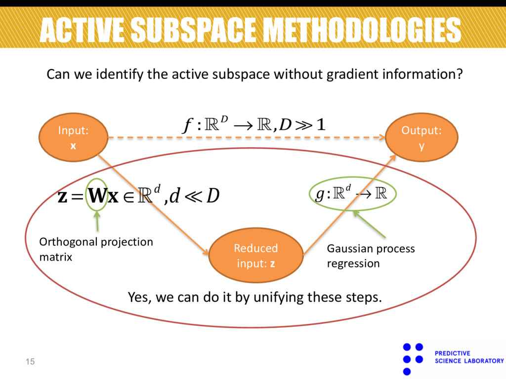
15. ACTIVE SUBSPACE METHODOLOGIES ! !g:!d → ! 15 Input: x Output: y ! !f :!D → !,D ≫1 Reduced input: z Orthogonal projection matrix Gaussian process regression ! ! !z = Wx ∈!d ,d ≪ D Can we identify the active subspace without gradient information? Yes, we can do it by unifying these steps.
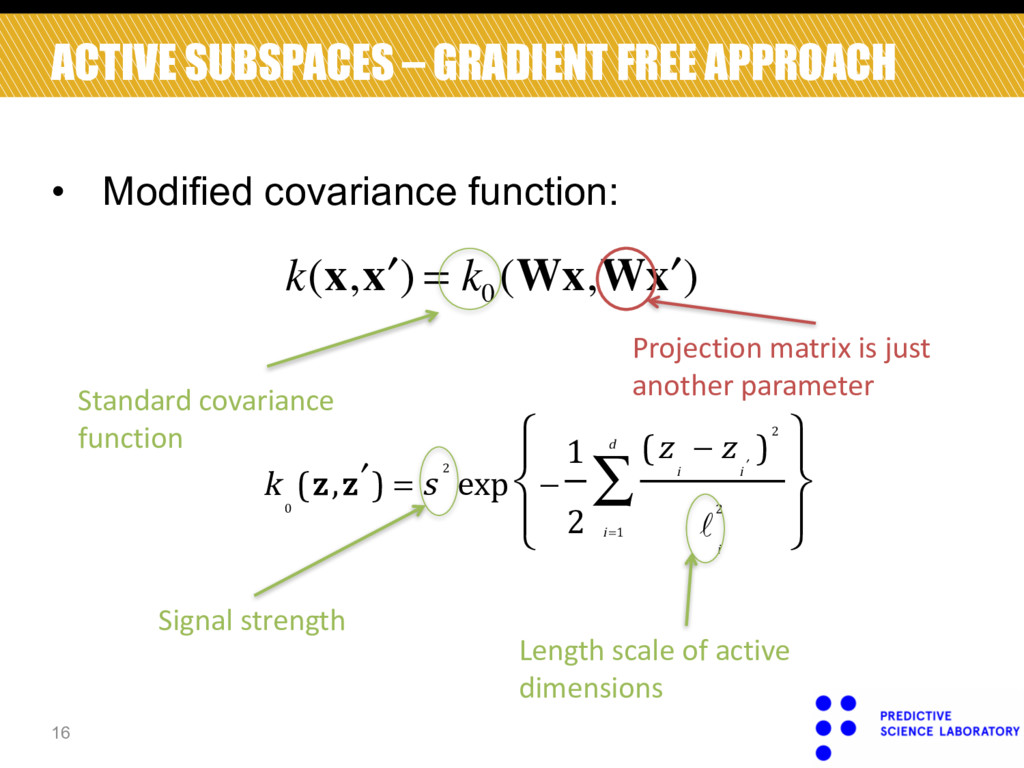
16. k(x, ′ x ) = k 0 (Wx,W ′ x ) ACTIVE SUBSPACES – GRADIENT FREE APPROACH • Modified covariance function: Standard covariance function ! ! ! k 0 $z, ′ z ' = s 2 exp − 1 2 $z i − z ′ i '2 ℓ i 2 i =1 d ∑ ⎧ ⎨ ⎩ ⎫ ⎬ ⎭ Signal strength Length scale of active dimensions 16 Projection matrix is just another parameter
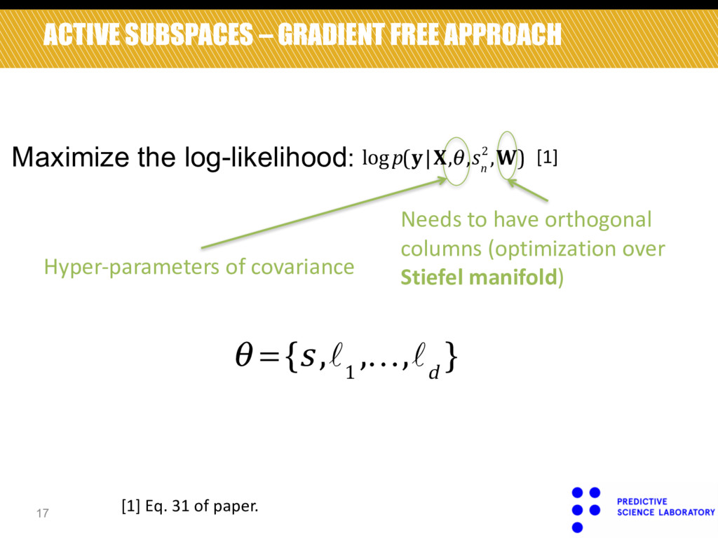
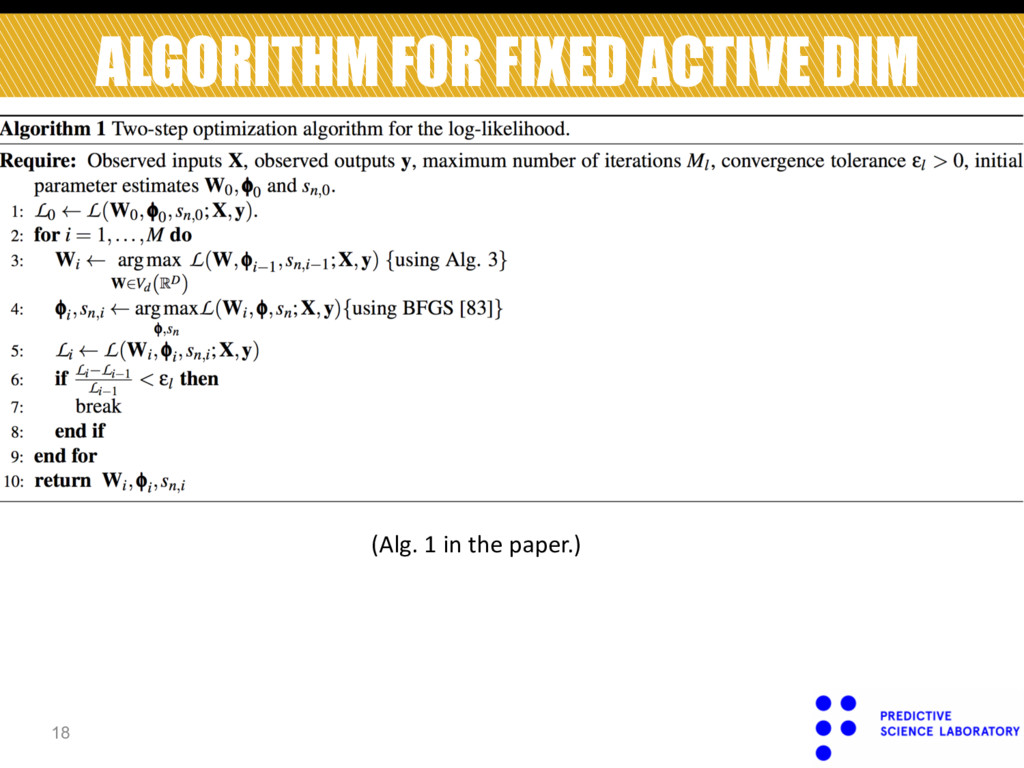
17. ACTIVE SUBSPACES – GRADIENT FREE APPROACH Maximize the log-likelihood: ! ! θ = "s,ℓ 1 ,…,ℓ d ' Hyper-parameters of covariance Needs to have orthogonal columns (optimization over Stiefel manifold) 17 logp(y|X,θ,s n 2 ,W) [1] [1] Eq. 31 of paper.
18. ALGORITHM FOR FIXED ACTIVE DIM 18 (Alg. 1 in the paper.)
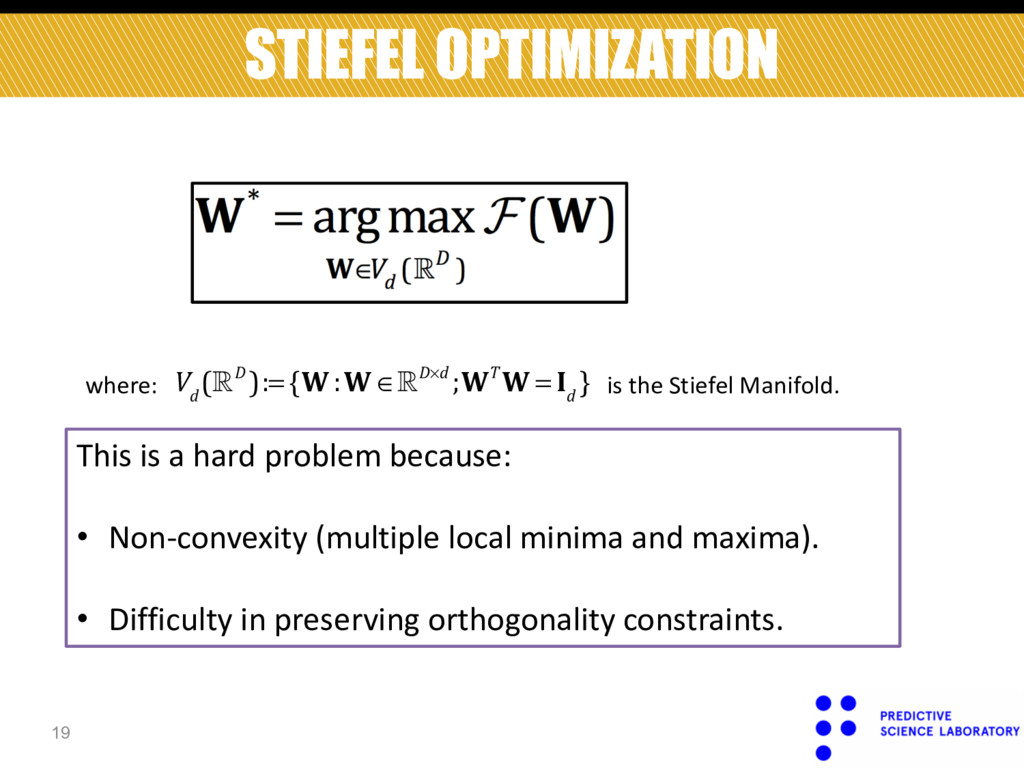
19. STIEFEL OPTIMIZATION 19 where: is the Stiefel Manifold. This is a hard problem because: • Non-convexity (multiple local minima and maxima). • Difficulty in preserving orthogonality constraints. V d (!D ):= {W:W ∈!D×d ;WTW = I d }
20. 20 STIEFEL OPTIMIZATION Gradient Ascent curve[1]: γ (τ;W)=(I D − τ 2 A(W))−1(I D + τ 2 A(W))W τ where, is the gradient-ascent step-size, A(W):= ∇ W F(W)W − W(∇ W F(W))T [1] Wen, Zaiwen, and Wotao Yin. "A feasible method for optimization with orthogonality constraints." Mathematical Programming 142.1-2 (2013) [2] Williams, Christopher KI, and Carl Edward Rasmussen. "Gaussian processes for machine learning." the MIT Press(2006)
21. 21 STIEFEL OPTIMIZATION (Alg. 3 in the paper) EGO Reference : Jones, Donald R., Matthias Schonlau, and William J. Welch. "Efficient global optimization of expensive black-box functions." Journal of Global optimization 13.4 (1998)
22. HOW DO WE PICK THE ACTIVE DIM? 22 Alg. 4 from paper
23. EX. 1 – SYNTHETIC RESPONSE SURFACE 23 f (x)= g(WT x) f :!D → ! s.t. Quadratic Link Function : g:!d → ! s.t. g(z)=α + βTz+zTΓz ∇f (x)=(β + xTWΓ)WT Gradients: α ∈!, β ∈!d , Γ ∈!d×d where:
24. 1-D ACTIVE SUBSPACE 24 Gradient-free approach Classic Approach Fig: Comparison of 1-d response surface when underlying AS is 1-d.
25. 1-D AS ( contd. ) 25 Gradient-free approach Classic Approach Fig: Comparison of 2-d response surface when underlying AS is 1-d.
26. 26 1-D AS ( contd. ) Gradient-free approach Classic Approach Fig: Comparison of projection matrix when underlying AS is 1-d.
27. 2-D ACTIVE SUBSPACE 27 Gradient-free approach Classic Approach Fig: Comparison of 1-d response surface when underlying AS is 2-d.
28. 2-D AS ( contd. ) 28 Gradient-free approach Classic Approach Fig: Comparison of 2-d response surface when underlying AS is 2-d.
29. 29 1-D AS ( contd. ) Gradient-free approach Classic Approach Fig: Comparison of projection matrix when underlying AS is 1-d.
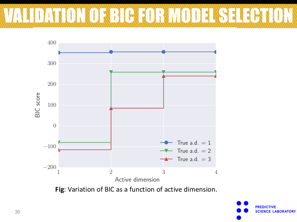
30. VALIDATION OF BIC FOR MODEL SELECTION 30 1 2 3 4 Active dimension 200 100 0 100 200 300 400 BIC score True a.d. = 1 True a.d. = 2 True a.d. = 3 Fig: Variation of BIC as a function of active dimension.
31. VALIDATION OF ROBUSTNESS TO NOISE 31 0.0 0.5 1.0 1.5 2.0 Noise variance, s2 n 10 4 10 3 10 2 10 1 100 101 Rel. error N = 30 N = 100 N = 200 N = 400 Fig: Robustness of proposed approach to observational noise.
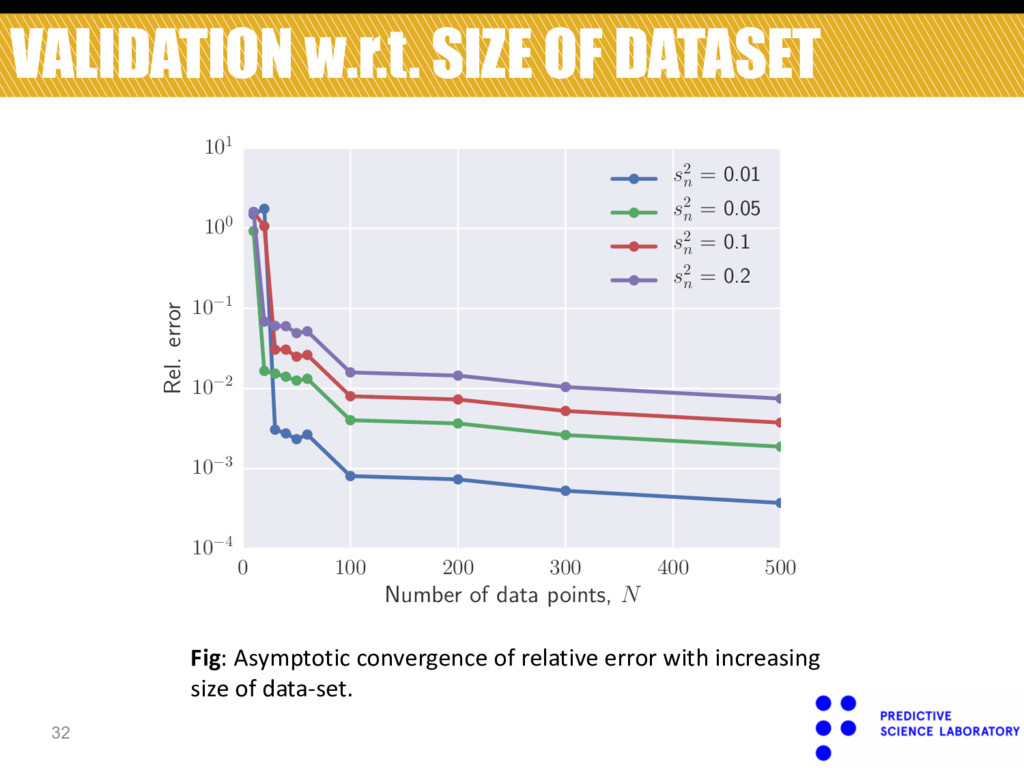
32. VALIDATION w.r.t. SIZE OF DATASET 32 0 100 200 300 400 500 Number of data points, N 10 4 10 3 10 2 10 1 100 101 Rel. error s2 n = 0.01 s2 n = 0.05 s2 n = 0.1 s2 n = 0.2 Fig: Asymptotic convergence of relative error with increasing size of data-set.
33. EX. 2 : ELLIPTIC PDE 33
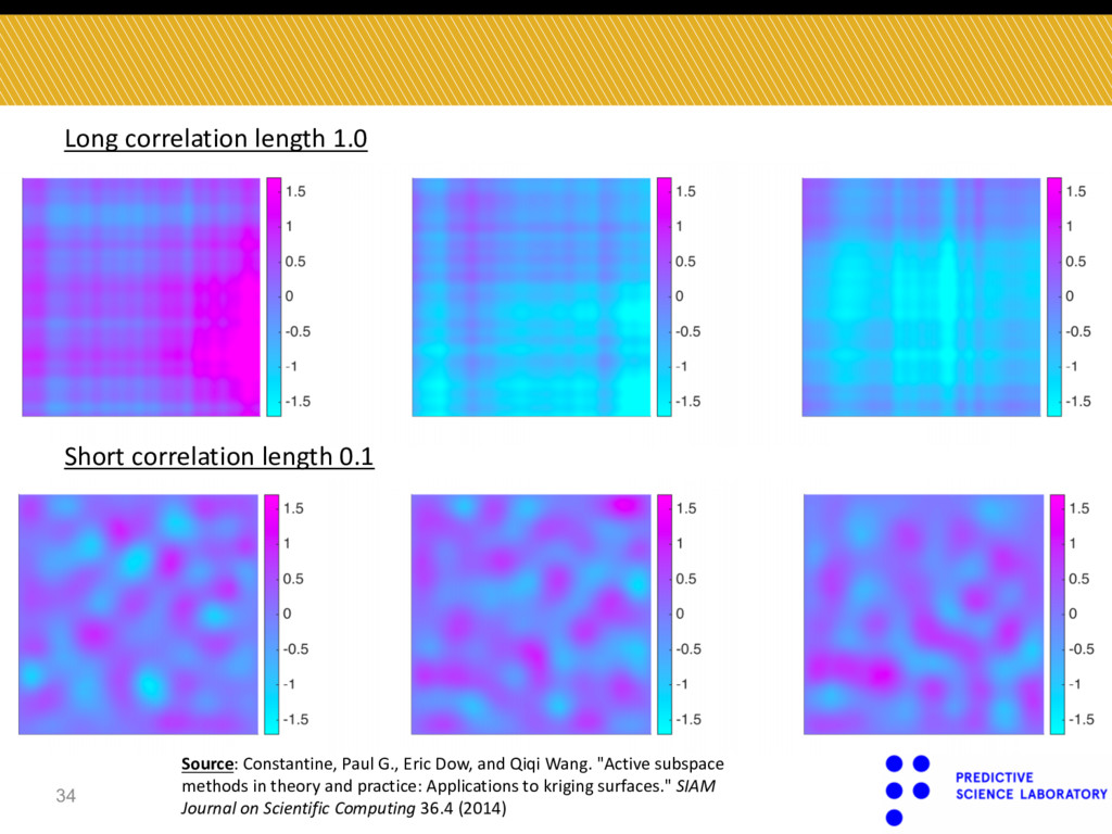
34. 34 Long correlation length 1.0 Short correlation length 0.1 Source: Constantine, Paul G., Eric Dow, and Qiqi Wang. "Active subspace methods in theory and practice: Applications to kriging surfaces." SIAM Journal on Scientific Computing 36.4 (2014)
35. RESULTS – LONG CORRELATION LENGTH 35 Gradient-free approach Classic Approach Fig: Comparison of 1-d response surface for long correlation length case.
36. RESULTS – LONG CORRELATION LENGTH 36 Gradient-free approach Classic Approach Fig: Comparison of 2-d response surface for long correlation length case.
37. RESULTS – LONG CORRELATION LENGTH 37 Gradient-free approach Classic Approach Fig: Comparison of projection matrix for long correlation length case.
38. RESULTS – SHORT CORRELATION LENGTH 38 Gradient-free approach Classic Approach Fig: Comparison of 1-d response surface for short correlation length case.
39. RESULTS – SHORT CORRELATION LENGTH 39 Gradient-free approach Classic Approach Fig: Comparison of projection matrix for short correlation length case.
40. PREDICTION VS OBSERVATION PLOTS 40 Short correlation length. Long correlation length. Fig: Pred. vs obs. plots for short and long correlation lengths using gradient-free approach.
41. GRANULAR CRYSTALS 41 • Unique, highly non-linear dynamical properties. • Formation and propagation of highly localized elastic stress waves. • Dynamics described by a fully elastic model known as the Hertz contact model.
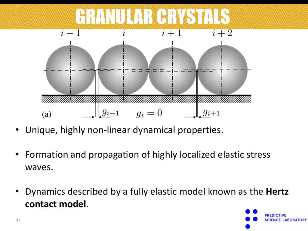
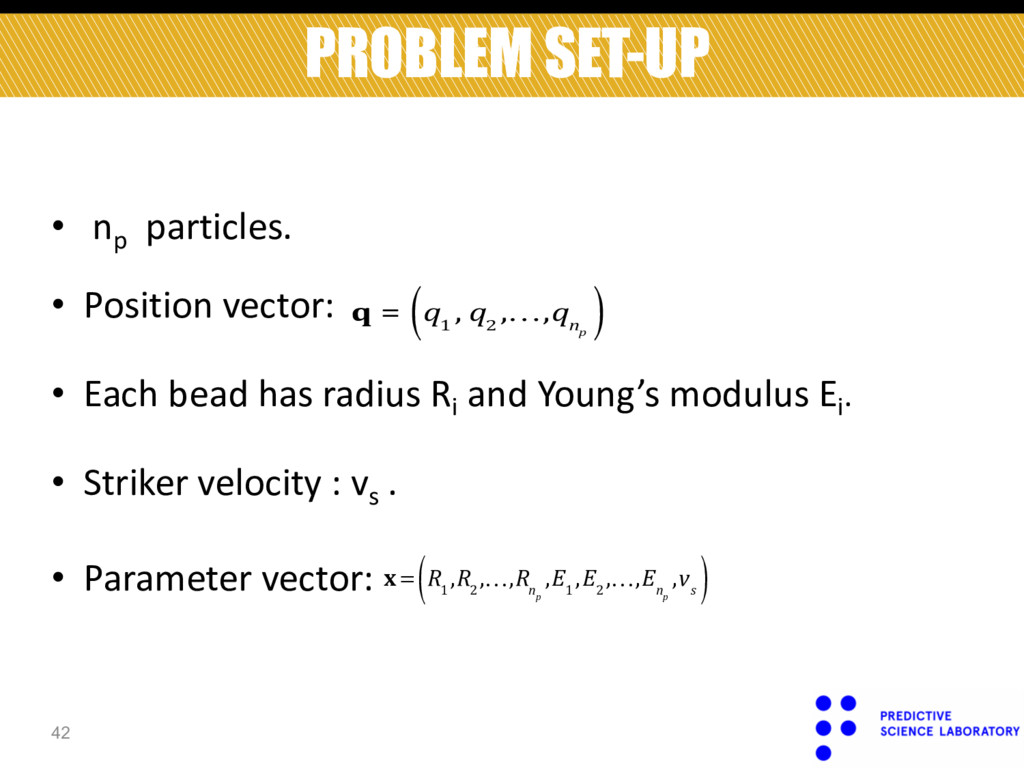
42. PROBLEM SET-UP 42 • np particles. • Position vector: • Each bead has radius Ri and Young’s modulus Ei . • Striker velocity : vs . • Parameter vector: q = q 1 , q 2 ,…,q n p ( ) x = R 1 ,R 2 ,…,R n p ,E 1 ,E 2 ,…,E n p ,v s ( )
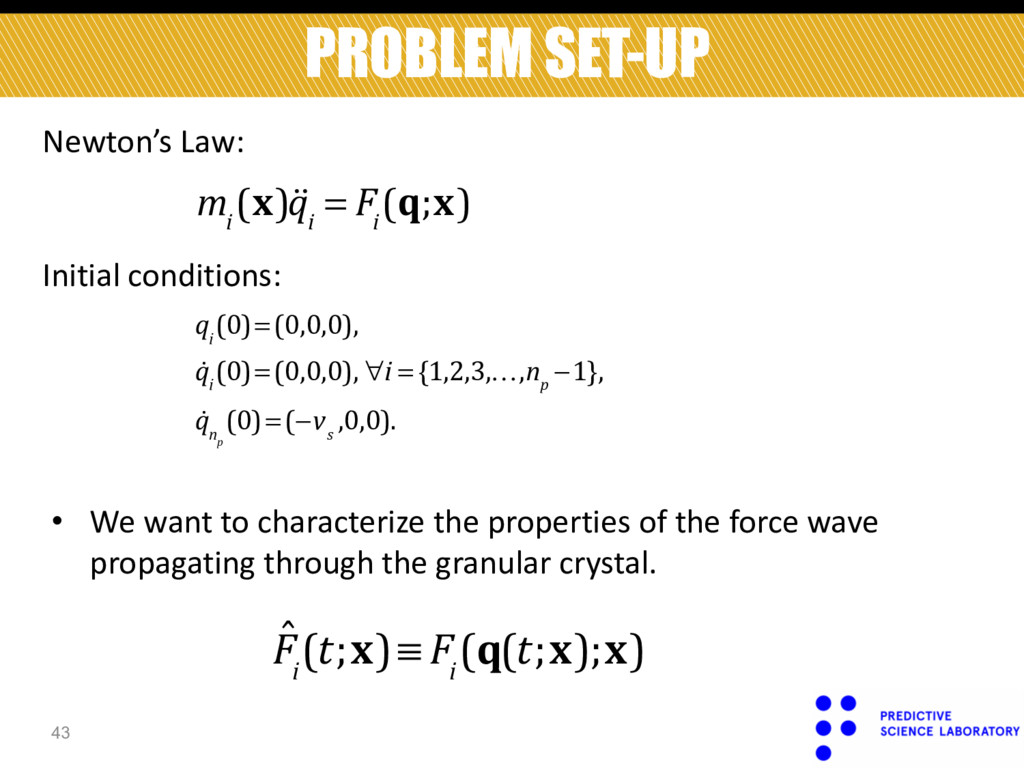
43. 43 PROBLEM SET-UP Newton’s Law: m i (x)!! q i = F i (q;x) Initial conditions: q i (0)=(0,0,0), ! q i (0)=(0,0,0), ∀i = {1,2,3,…,n p −1}, ! q n p (0)=(−v s ,0,0). • We want to characterize the properties of the force wave propagating through the granular crystal. ˆ F i (t;x)≡ F i (q(t;x);x)
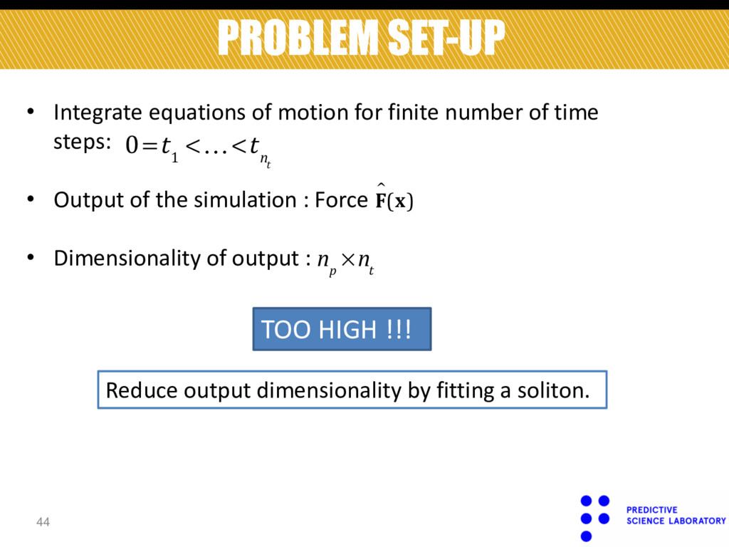
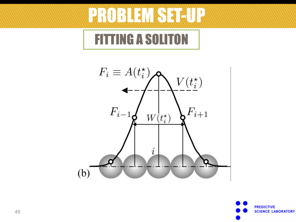
44. 44 PROBLEM SET-UP • Integrate equations of motion for finite number of time steps: • Output of the simulation : Force • Dimensionality of output : 0=t 1 <…<t n t F !(x) n p ×n t TOO HIGH !!! Reduce output dimensionality by fitting a soliton.
45. 45 FITTING A SOLITON PROBLEM SET-UP
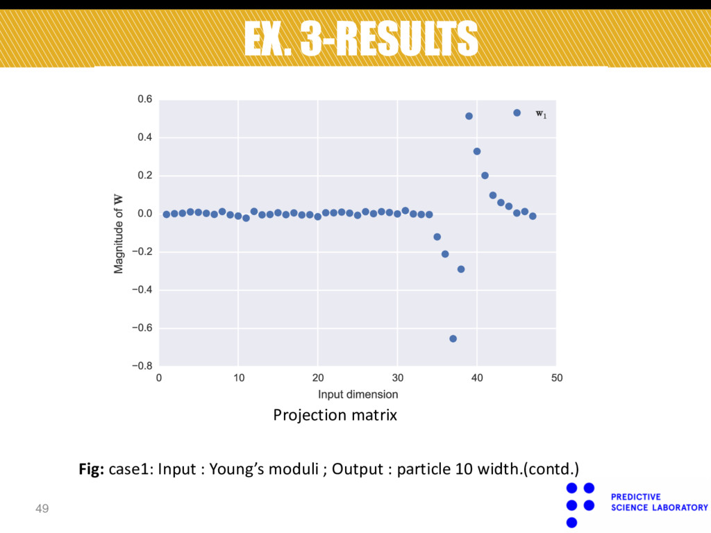
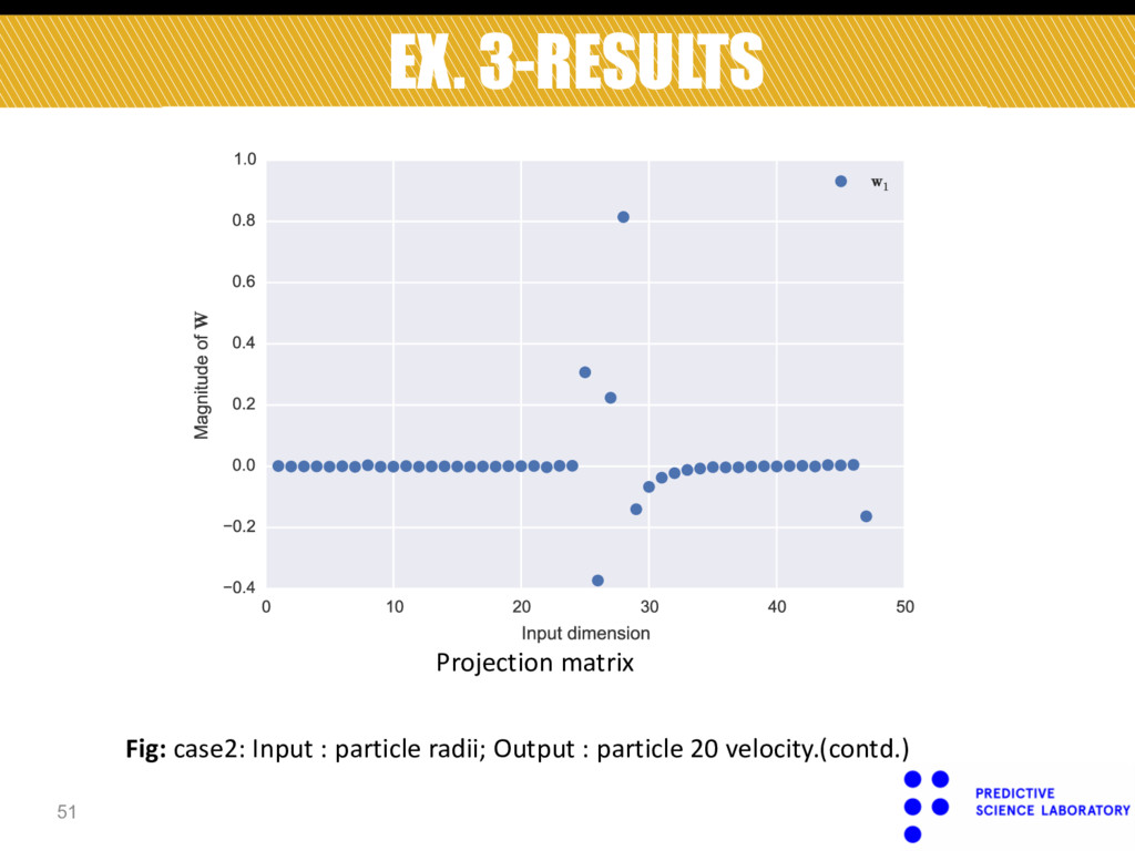
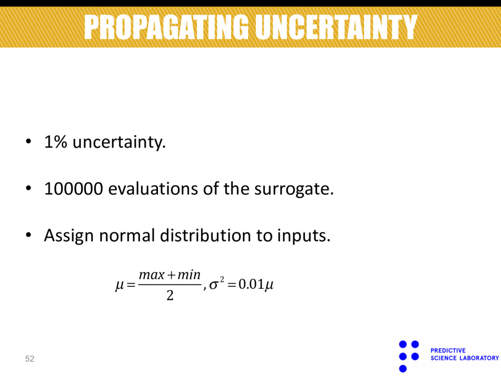
47. EX. 3-RESULTS 47 • Particles 10 and 20. • Specifically we show results for the following 3 cases: § Input=Young’s modulus, Output=width over 10th particle. § Input=particle radii, Output=velocity over 20th particle.
48. 48 EX. 3-RESULTS Response surface (1-d) Pred. vs obs. Fig: case1: Input : Young’s moduli ; Output : particle 10 width.
49. 49 EX. 3-RESULTS Projection matrix Fig: case1: Input : Young’s moduli ; Output : particle 10 width.(contd.)
50. 50 EX. 3-RESULTS Response surface (1-d) Pred. vs obs. Fig: case2: Input : particle radii; Output : particle 20 velocity.
51. 51 EX. 3-RESULTS Projection matrix Fig: case2: Input : particle radii; Output : particle 20 velocity.(contd.)
52. PROPAGATING UNCERTAINTY 52 • 1% uncertainty. • 100000 evaluations of the surrogate. • Assign normal distribution to inputs. µ = max +min 2 ,σ 2 = 0.01µ
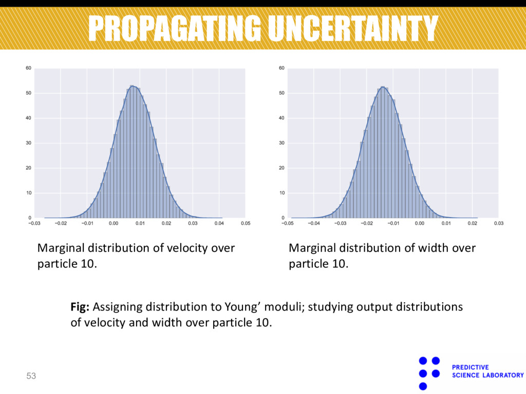
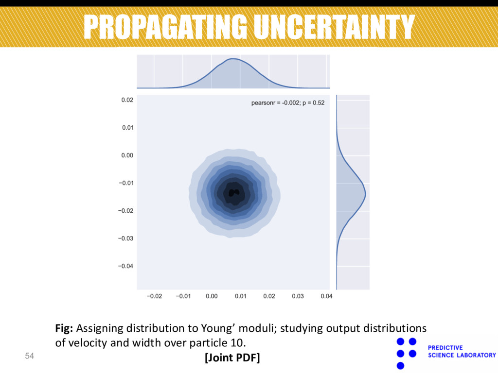
53. 53 PROPAGATING UNCERTAINTY Marginal distribution of width over particle 10. Marginal distribution of velocity over particle 10. Fig: Assigning distribution to Young’ moduli; studying output distributions of velocity and width over particle 10.
54. 54 PROPAGATING UNCERTAINTY Fig: Assigning distribution to Young’ moduli; studying output distributions of velocity and width over particle 10. [Joint PDF]
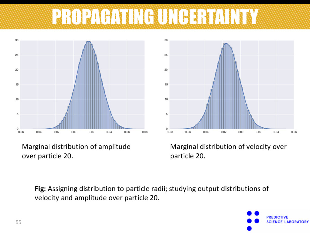
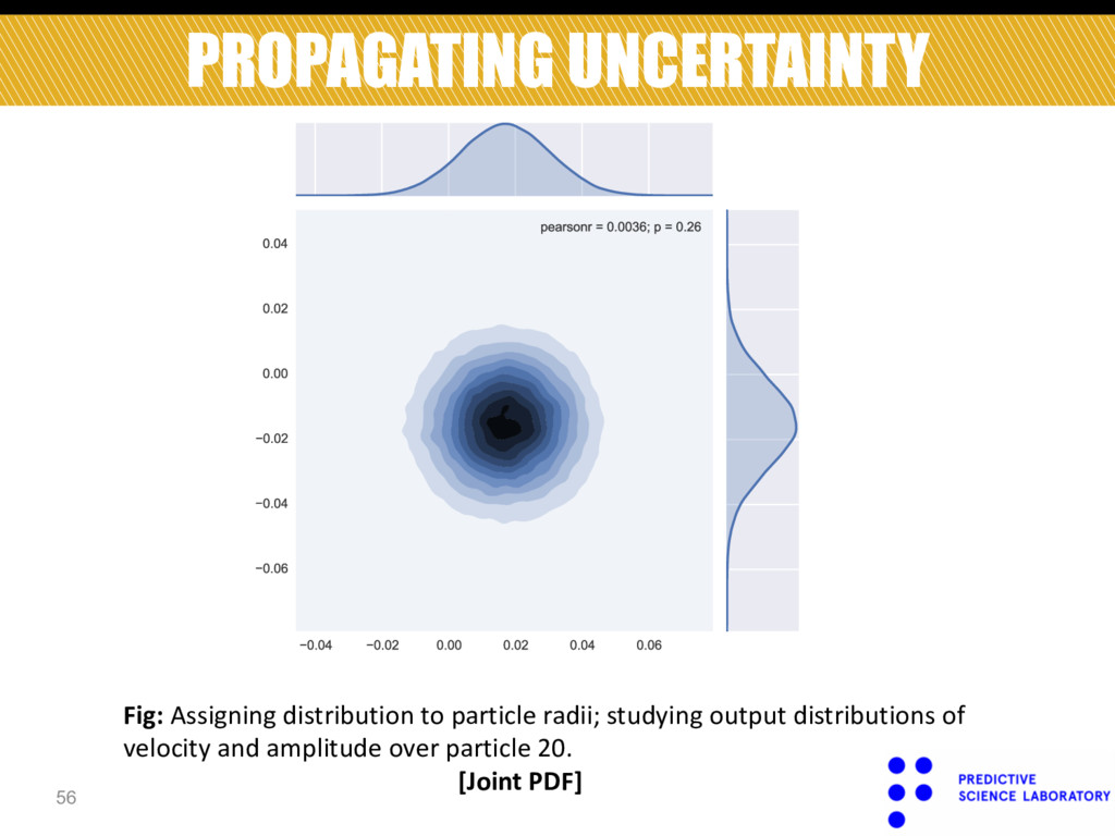
55. 55 PROPAGATING UNCERTAINTY Marginal distribution of velocity over particle 20. Marginal distribution of amplitude over particle 20. Fig: Assigning distribution to particle radii; studying output distributions of velocity and amplitude over particle 20.
56. 56 PROPAGATING UNCERTAINTY Fig: Assigning distribution to particle radii; studying output distributions of velocity and amplitude over particle 20. [Joint PDF]
57. CONCLUSIONS AND FUTURE WORK 57 • Gradient-free approach to AS discovery. • Novel Gaussian process regression with built-in dimensionality reduction. • Orthogonal projection matrix which constitutes a hyper- parameter of the covariance kernel. • BIC score for model selection. • Validated methodology through 3 numerical examples.
58. 58 CONCLUSIONS AND FUTURE WORK • First step toward fully Bayesian AS-based surrogate. • Fully Bayesian treatment ; specification of priors for all hyper- parameters. • Derivation of MCMC scheme. • Non-linear low-dimensional manifold.