Evangelos Vlachos - Successive ICI Cancellation based on Galerkin Projections for OFDM Systems in Doubly Selective Channels

Transcript

1. Introduction Slow Fading Fast Fading Conclusions Successive ICI Cancellation based on Galerkin Projections for OFDM Systems in Doubly Selective Channels Evangelos Vlachos Ph.D candidate, vlaxose@ceid.upatras.gr Signal Processing and Communications Laboratory Department of Computer Engineering and Informatics University of Patras, Greece
2. Introduction Slow Fading Fast Fading Conclusions Outline Introduction Slow Fading Doubly Selective Channels Problem formulation ICI equalization techniques Regularized MMSE equalization Fast Fading Doubly Selective Channels Simulation Studies Problem formulation Successive ICI Mitigation Techniques Galerkin Projections SIC Simulation Studies Conclusions
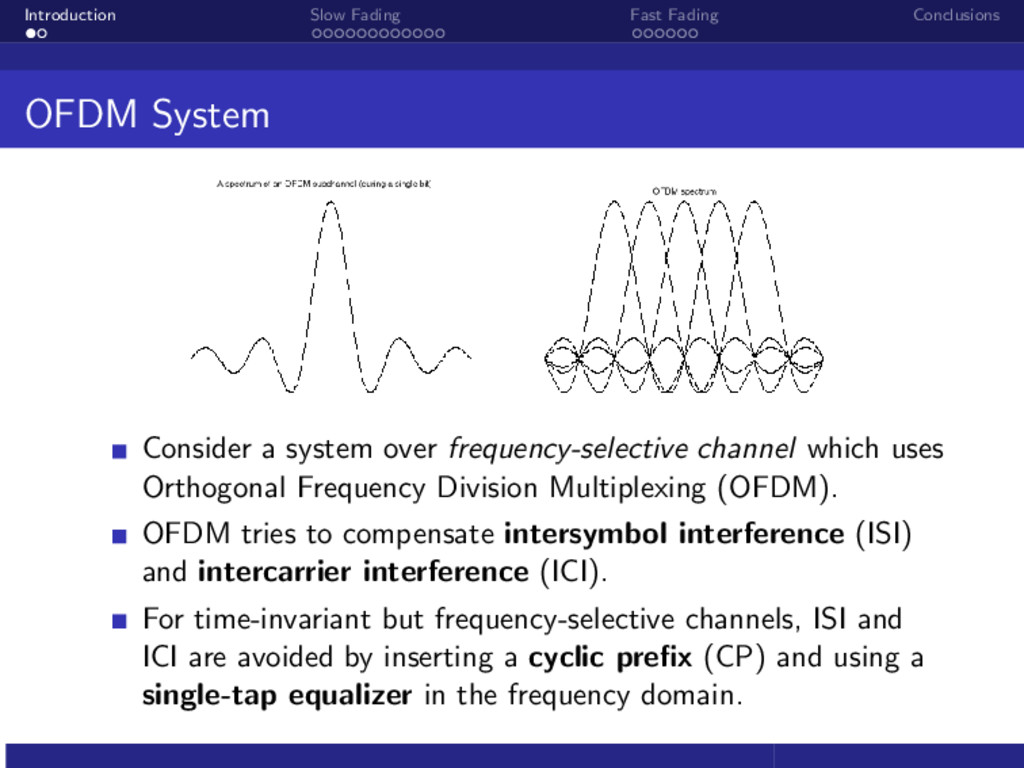
3. Introduction Slow Fading Fast Fading Conclusions OFDM System Consider a system over frequency-selective channel which uses Orthogonal Frequency Division Multiplexing (OFDM). OFDM tries to compensate intersymbol interference (ISI) and intercarrier interference (ICI). For time-invariant but frequency-selective channels, ISI and ICI are avoided by inserting a cyclic prefix (CP) and using a single-tap equalizer in the frequency domain.
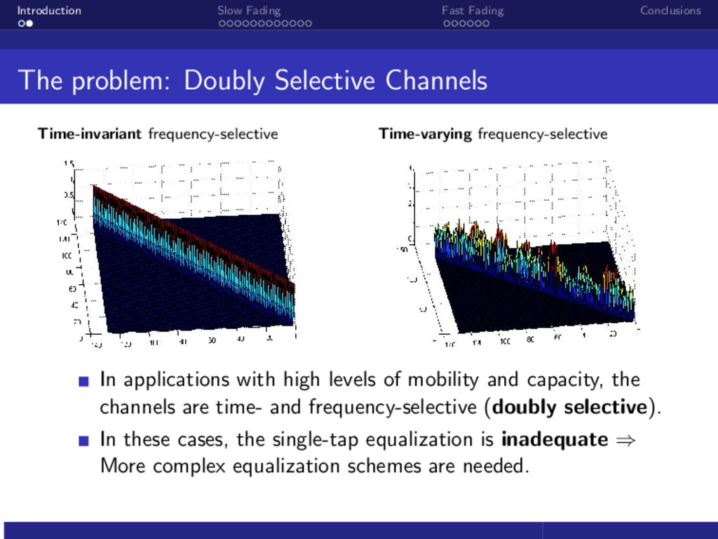
4. Introduction Slow Fading Fast Fading Conclusions The problem: Doubly Selective Channels Time-invariant frequency-selective Time-varying frequency-selective In applications with high levels of mobility and capacity, the channels are time- and frequency-selective (doubly selective). In these cases, the single-tap equalization is inadequate ⇒ More complex equalization schemes are needed.
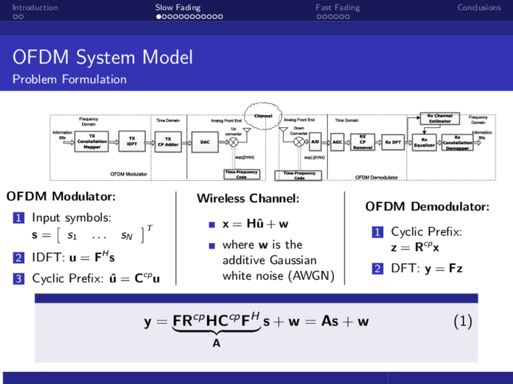
5. Introduction Slow Fading Fast Fading Conclusions OFDM System Model Problem Formulation OFDM Modulator: 1 Input symbols: s = s1 . . . sN T 2 IDFT: u = FH s 3 Cyclic Prefix: ˆ u = Ccpu Wireless Channel: x = Hˆ u + w where w is the additive Gaussian white noise (AWGN) OFDM Demodulator: 1 Cyclic Prefix: z = Rcpx 2 DFT: y = Fz y = FRcpHCcpFH A s + w = As + w (1)
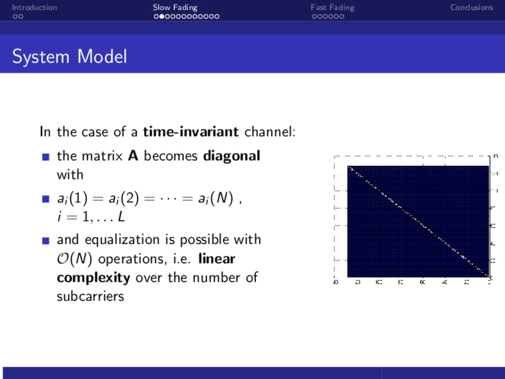
6. Introduction Slow Fading Fast Fading Conclusions System Model In the case of a time-invariant channel: the matrix A becomes diagonal with ai (1) = ai (2) = · · · = ai (N) , i = 1, . . . L and equalization is possible with O(N) operations, i.e. linear complexity over the number of subcarriers
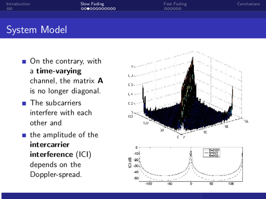
7. Introduction Slow Fading Fast Fading Conclusions System Model On the contrary, with a time-varying channel, the matrix A is no longer diagonal. The subcarriers interfere with each other and the amplitude of the intercarrier interference (ICI) depends on the Doppler-spread.
8. Introduction Slow Fading Fast Fading Conclusions Conventional MMSE Equalizer Apply the MMSE equalization to the parallel N streams, i.e. solve N systems of equations of N × N, hence O(N3) total complexity. The MMSE equalization matrix is given by the solution of E{yyH }G = E{syH } (2) ⇒ RG = B (3) ⇒    r11 r12 . . . r1N . . . . . . . . . . . . rN1 rN2 . . . rNN       g11 g12 . . . g1N . . . . . . . . . . . . gN1 gN2 . . . gNN    =    b11 b12 . . . b1N . . . . . . . . . . . . bN1 bN2 . . . bNN    ( where G is the equalizer matrix G = [g1g2 . . . gN]T .
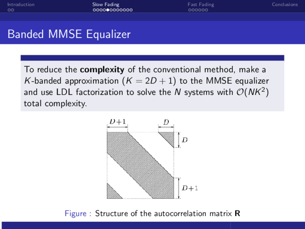
9. Introduction Slow Fading Fast Fading Conclusions Banded MMSE Equalizer To reduce the complexity of the conventional method, make a K-banded approximation (K = 2D + 1) to the MMSE equalizer and use LDL factorization to solve the N systems with O(NK2) total complexity. Figure : Structure of the autocorrelation matrix R
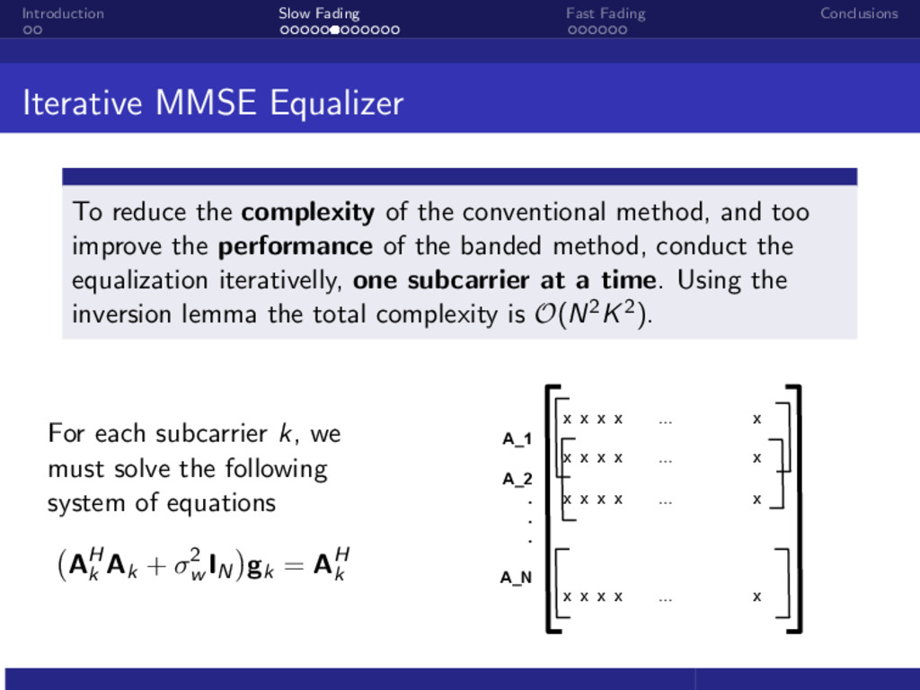
10. Introduction Slow Fading Fast Fading Conclusions Iterative MMSE Equalizer To reduce the complexity of the conventional method, and too improve the performance of the banded method, conduct the equalization iterativelly, one subcarrier at a time. Using the inversion lemma the total complexity is O(N2K2). For each subcarrier k, we must solve the following system of equations AH k Ak + σ2 w IN gk = AH k x x x x ... x x x x x ... x x x x x ... x x x x x ... x A_1 A_2 . . . A_N
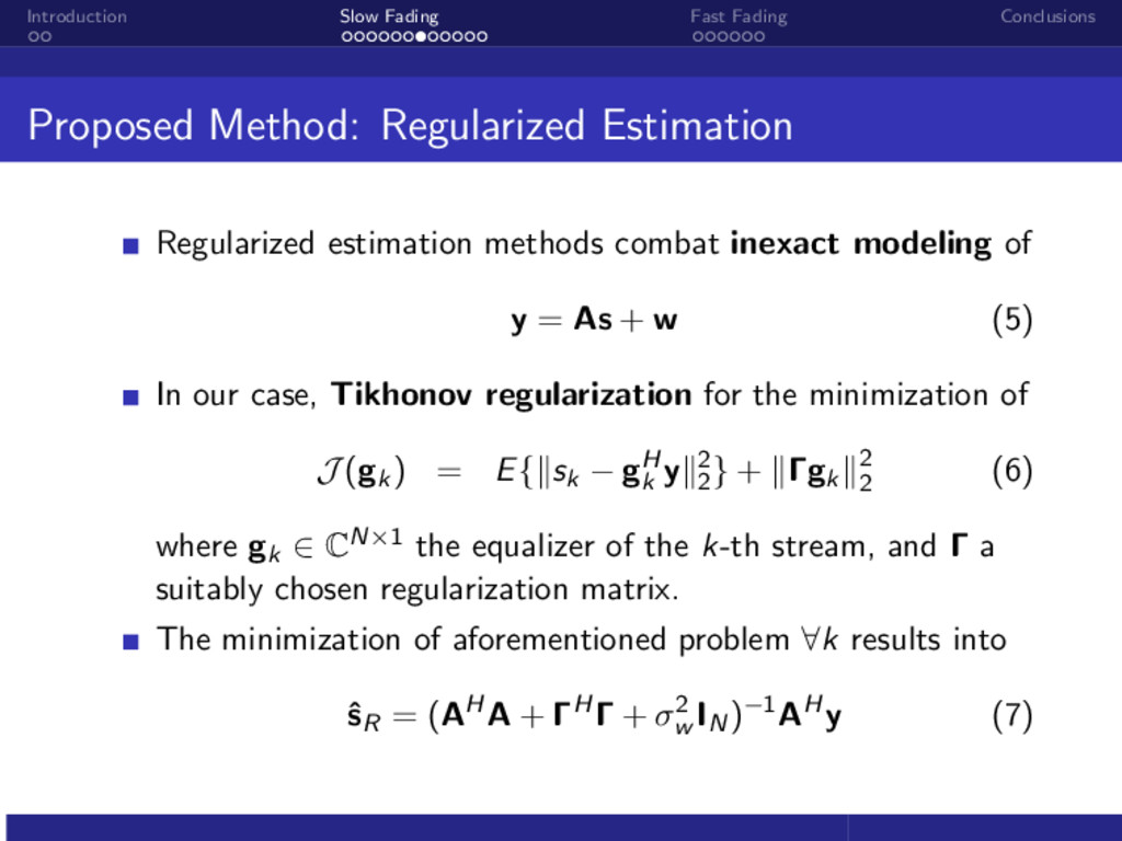
11. Introduction Slow Fading Fast Fading Conclusions Proposed Method: Regularized Estimation Regularized estimation methods combat inexact modeling of y = As + w (5) In our case, Tikhonov regularization for the minimization of J (gk) = E{ sk − gH k y 2 2 } + Γgk 2 2 (6) where gk ∈ CN×1 the equalizer of the k-th stream, and Γ a suitably chosen regularization matrix. The minimization of aforementioned problem ∀k results into ˆ sR = (AHA + ΓHΓ + σ2 w IN)−1AHy (7)
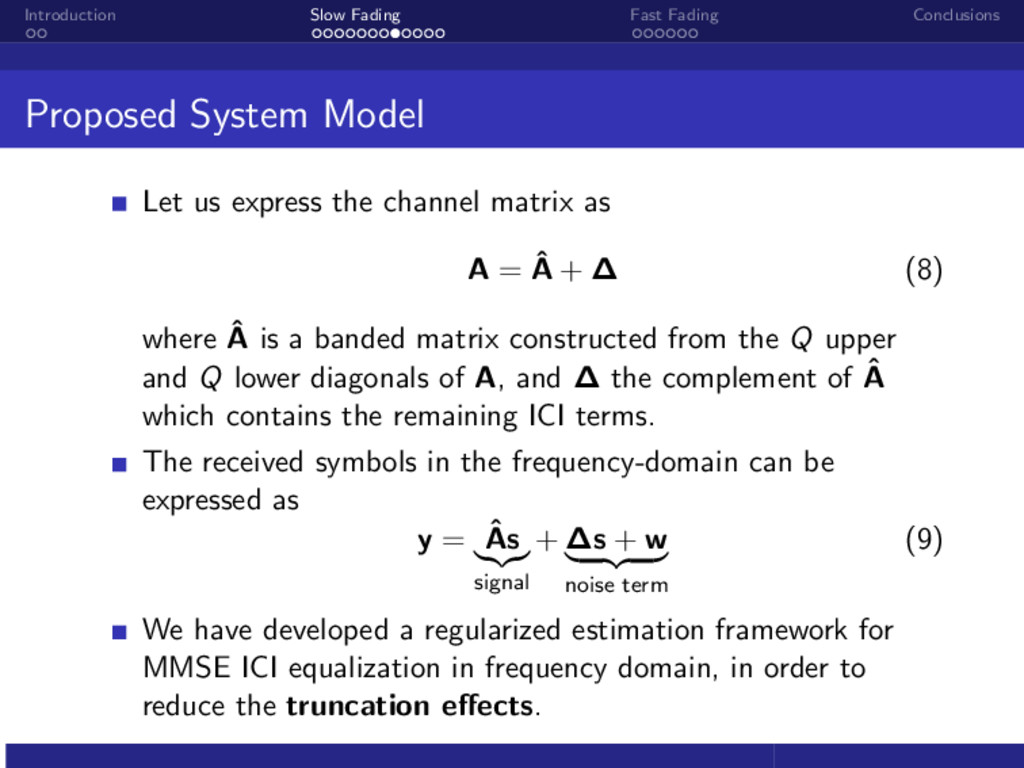
12. Introduction Slow Fading Fast Fading Conclusions Proposed System Model Let us express the channel matrix as A = ˆ A + ∆ (8) where ˆ A is a banded matrix constructed from the Q upper and Q lower diagonals of A, and ∆ the complement of ˆ A which contains the remaining ICI terms. The received symbols in the frequency-domain can be expressed as y = ˆ As signal + ∆s + w noise term (9) We have developed a regularized estimation framework for MMSE ICI equalization in frequency domain, in order to reduce the truncation effects.
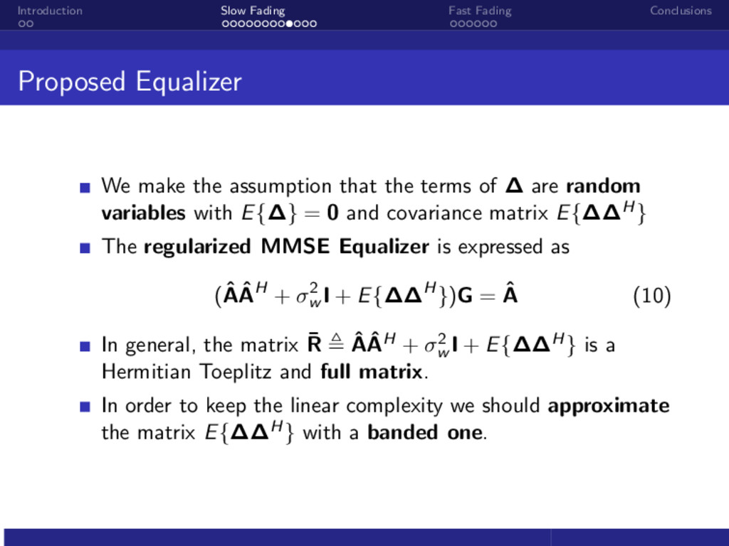
13. Introduction Slow Fading Fast Fading Conclusions Proposed Equalizer We make the assumption that the terms of ∆ are random variables with E{∆} = 0 and covariance matrix E{∆∆H} The regularized MMSE Equalizer is expressed as (ˆ Aˆ AH + σ2 w I + E{∆∆H})G = ˆ A (10) In general, the matrix ¯ R ˆ Aˆ AH + σ2 w I + E{∆∆H} is a Hermitian Toeplitz and full matrix. In order to keep the linear complexity we should approximate the matrix E{∆∆H} with a banded one.
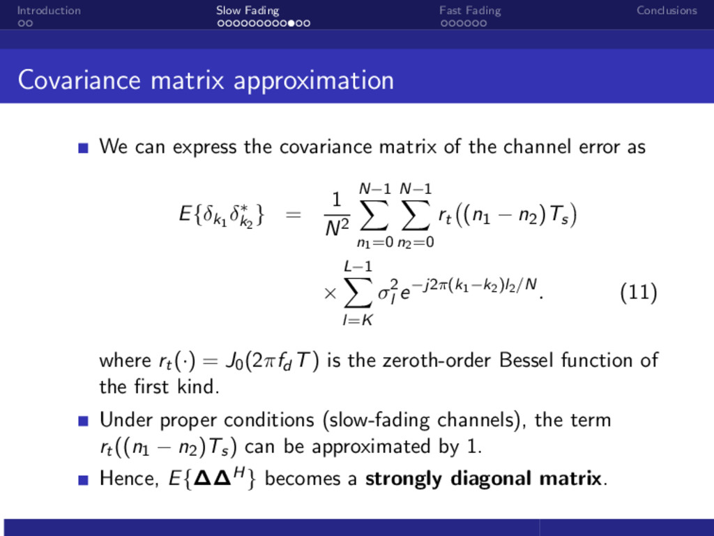
14. Introduction Slow Fading Fast Fading Conclusions Covariance matrix approximation We can express the covariance matrix of the channel error as E{δk1 δ∗ k2 } = 1 N2 N−1 n1=0 N−1 n2=0 rt (n1 − n2)Ts × L−1 l=K σ2 l e−j2π(k1−k2)l2/N. (11) where rt(·) = J0(2πfd T) is the zeroth-order Bessel function of the first kind. Under proper conditions (slow-fading channels), the term rt((n1 − n2)Ts) can be approximated by 1. Hence, E{∆∆H} becomes a strongly diagonal matrix.
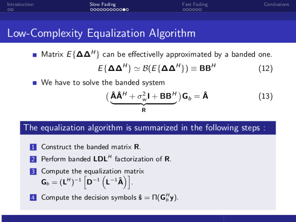
15. Introduction Slow Fading Fast Fading Conclusions Low-Complexity Equalization Algorithm Matrix E{∆∆H } can be effectivelly approximated by a banded one. E{∆∆H } B(E{∆∆H }) ≡ BBH (12) We have to solve the banded system ˆ Aˆ AH + σ2 w I + BBH R Gb = ˆ A (13) The equalization algorithm is summarized in the following steps : 1 Construct the banded matrix R. 2 Perform banded LDLH factorization of R. 3 Compute the equalization matrix Gb = (LH )−1 D−1 L−1 ˆ A . 4 Compute the decision symbols ˆ s = Π(GH b y).
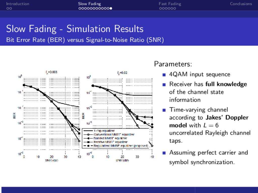
16. Introduction Slow Fading Fast Fading Conclusions Slow Fading - Simulation Results Bit Error Rate (BER) versus Signal-to-Noise Ratio (SNR) Parameters: 4QAM input sequence Receiver has full knowledge of the channel state information Time-varying channel according to Jakes’ Doppler model with L = 6 uncorrelated Rayleigh channel taps. Assuming perfect carrier and symbol synchronization.
17. Introduction Slow Fading Fast Fading Conclusions Successive MMSE Cancellation Successive cancellation offers effective ICI mitigation. Detecting the date one-by-one we utilize the time diversity. Each subcarrier is associated with one of the N transmitted symbols. At a given iteration, we can subtract the already decided symbols/subcarriers.
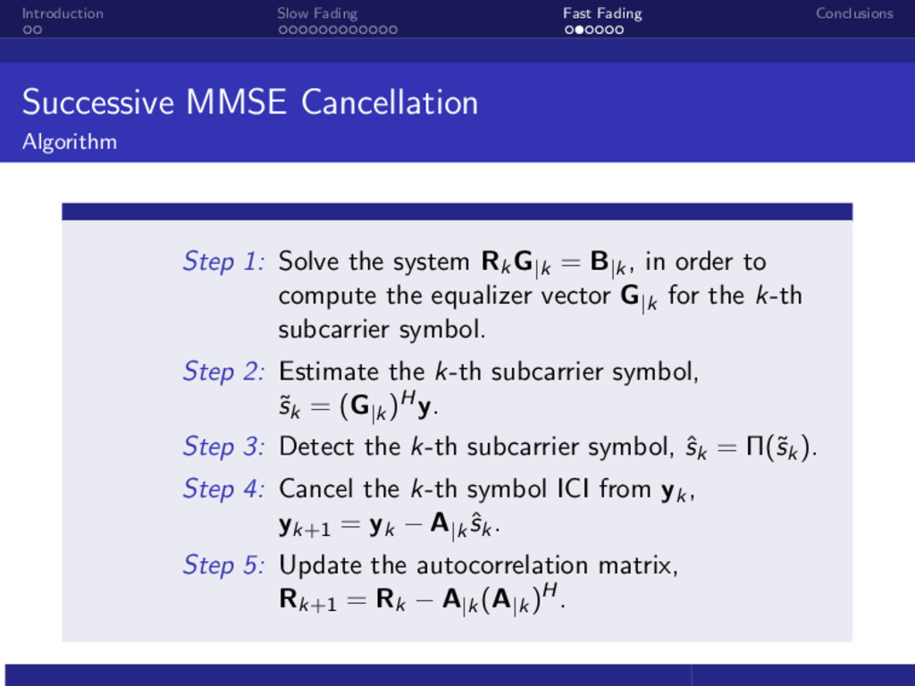
18. Introduction Slow Fading Fast Fading Conclusions Successive MMSE Cancellation Algorithm Step 1: Solve the system RkG|k = B|k , in order to compute the equalizer vector G|k for the k-th subcarrier symbol. Step 2: Estimate the k-th subcarrier symbol, ˜ sk = (G|k )Hy. Step 3: Detect the k-th subcarrier symbol, ˆ sk = Π(˜ sk). Step 4: Cancel the k-th symbol ICI from yk, yk+1 = yk − A|k ˆ sk. Step 5: Update the autocorrelation matrix, Rk+1 = Rk − A|k (A|k )H.
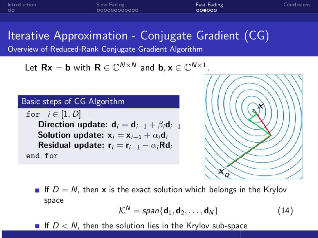
19. Introduction Slow Fading Fast Fading Conclusions Iterative Approximation - Conjugate Gradient (CG) Overview of Reduced-Rank Conjugate Gradient Algorithm Let Rx = b with R ∈ CN×N and b, x ∈ CN×1. Basic steps of CG Algorithm for i ∈ [1, D] Direction update: di = di−1 + βi di−1 Solution update: xi = xi−1 + αi di Residual update: ri = ri−1 − αi Rdi end for If D = N, then x is the exact solution which belongs in the Krylov space KN = span{d1, d2, . . . , dN } (14) If D < N, then the solution lies in the Krylov sub-space
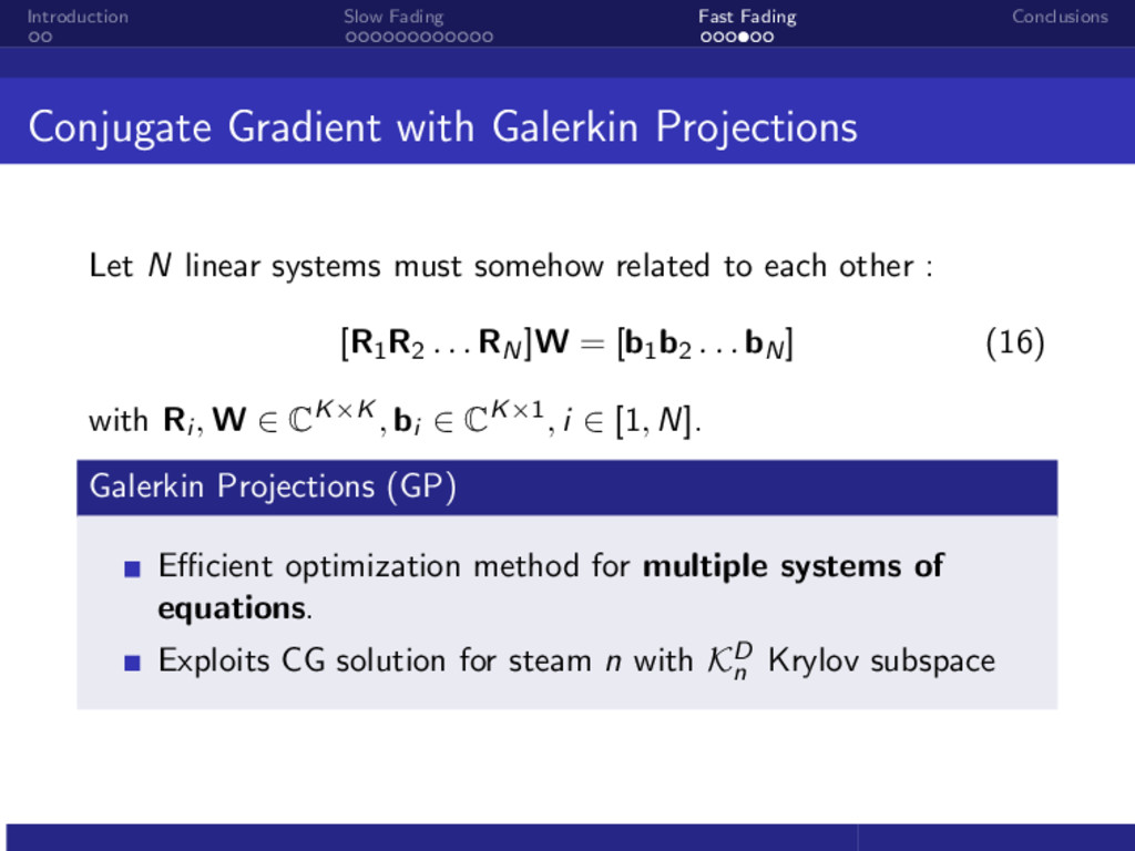
20. Introduction Slow Fading Fast Fading Conclusions Conjugate Gradient with Galerkin Projections Let N linear systems must somehow related to each other : [R1R2 . . . RN]W = [b1b2 . . . bN] (16) with Ri , W ∈ CK×K , bi ∈ CK×1, i ∈ [1, N]. Galerkin Projections (GP) Efficient optimization method for multiple systems of equations. Exploits CG solution for steam n with KD n Krylov subspace
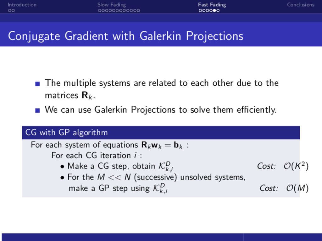
21. Introduction Slow Fading Fast Fading Conclusions Conjugate Gradient with Galerkin Projections The multiple systems are related to each other due to the matrices Rk. We can use Galerkin Projections to solve them efficiently. CG with GP algorithm For each system of equations Rk wk = bk : For each CG iteration i : • Make a CG step, obtain KD k,i Cost: O(K2) • For the M << N (successive) unsolved systems, make a GP step using KD k,i Cost: O(M)
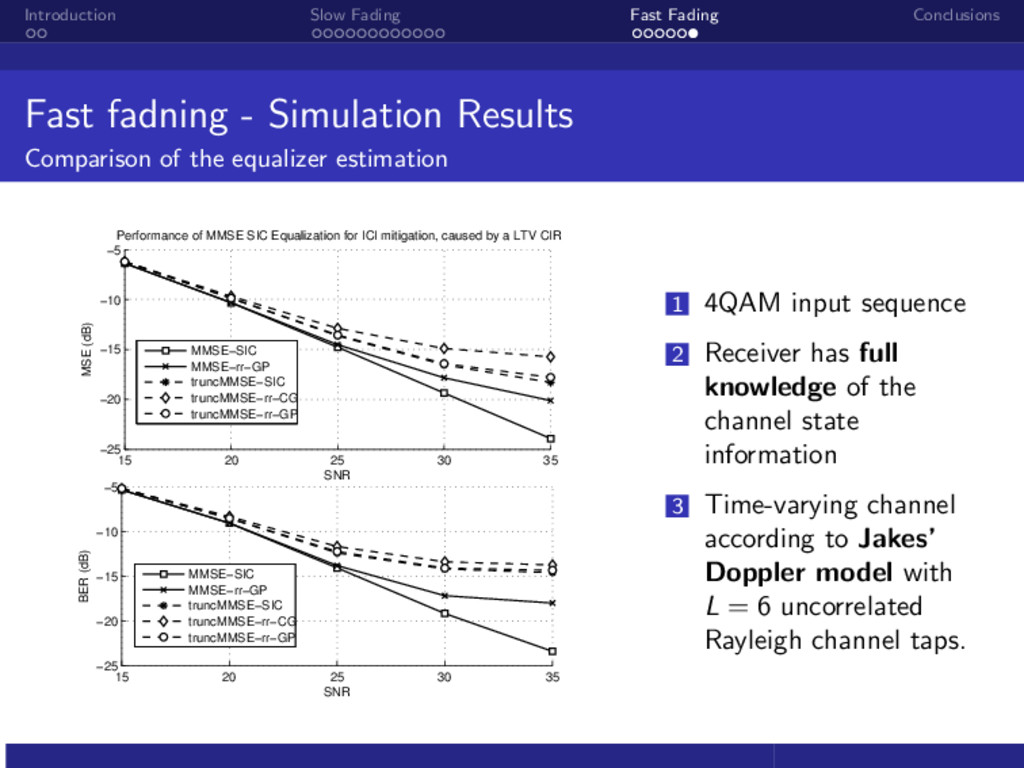
22. Introduction Slow Fading Fast Fading Conclusions Fast fadning - Simulation Results Comparison of the equalizer estimation 15 20 25 30 35 −25 −20 −15 −10 −5 SNR MSE (dB) Performance of MMSE SIC Equalization for ICI mitigation, caused by a LTV CIR MMSE−SIC MMSE−rr−GP truncMMSE−SIC truncMMSE−rr−CG truncMMSE−rr−GP 15 20 25 30 35 −25 −20 −15 −10 −5 SNR BER (dB) MMSE−SIC MMSE−rr−GP truncMMSE−SIC truncMMSE−rr−CG truncMMSE−rr−GP 1 4QAM input sequence 2 Receiver has full knowledge of the channel state information 3 Time-varying channel according to Jakes’ Doppler model with L = 6 uncorrelated Rayleigh channel taps.
23. Introduction Slow Fading Fast Fading Conclusions Conclusions The ICI is introduced at the receiver due to doubly selective channel. For slow fading channels (small Doppler-spread) the linear equalization is adequate with low-complexity. We have described a regularized MMSE equalizer which accounts the inexact modeling, and through simulation results have been verified that recovers the lost performance while the complexity remains linear. For fast fading (large Doppler-spread), a canellation method (SIC) must be used, which has increased complexity. We have described a CG-based SIC technique has been derived here and has been further improved by proper use of Galerkin projections theory.
24. Introduction Slow Fading Fast Fading Conclusions Conclusions Thank you for your attention!