New Horizons In Gravitational-wave Astronomy With Pulsar-Timing Arrays

[07/19/2016] Seminar given at Armagh Observatory, Northern Ireland.

Transcript

1. Stephen Taylor Armagh Observatory, 07/19/2016 © 2016 California Institute of Technology. Government sponsorship acknowledged Stephen R. Taylor New Horizons In Gravitational-wave Astronomy With Pulsar-Timing Arrays NASA POSTDOCTORAL FELLOW, JET PROPULSION LABORATORY, CALIFORNIA INSTITUTE OF TECHNOLOGY
2. Stephen Taylor Armagh Observatory, 07/19/2016 Gravitational waves ! The gravitational-wave spectrum [ LIGO, (e)LISA, PTAs ] ! Pulsars and pulsar-timing ! Searching for nanohertz GWs Overview
3. Stephen Taylor Armagh Observatory, 07/19/2016 Gravitational waves Perturbation to space-time metric. ! Sourced by accelerating masses. ! Any dynamical system with accelerating quadrupole moment produces GWs.
4. Stephen Taylor Armagh Observatory, 07/19/2016 Gravitational waves Perturbation to space-time metric. ! Sourced by accelerating masses. ! Any dynamical system with accelerating quadrupole moment produces GWs.
5. Stephen Taylor Armagh Observatory, 07/19/2016 Gravitational waves Perturbation to space-time metric. ! Sourced by accelerating masses. ! Any dynamical system with accelerating quadrupole moment produces GWs.
6. Stephen Taylor Armagh Observatory, 07/19/2016 The SXS (Simulating eXtreme Spacetimes) Project Gravitational waves
7. Stephen Taylor Armagh Observatory, 07/19/2016 The SXS (Simulating eXtreme Spacetimes) Project Gravitational waves
8. Stephen Taylor Armagh Observatory, 07/19/2016 http://rhcole.com/apps/GWplotter.
9. Stephen Taylor Armagh Observatory, 07/19/2016 LIGO/T. Pyle The GW spectrum [LIGO]
10. Stephen Taylor Armagh Observatory, 07/19/2016 LIGO/T. Pyle The GW spectrum [LIGO]
11. Stephen Taylor Armagh Observatory, 07/19/2016 LIGO The GW spectrum [LIGO]
12. Stephen Taylor Armagh Observatory, 07/19/2016 LIGO The GW spectrum [LIGO]
13. Stephen Taylor Armagh Observatory, 07/19/2016 The GW spectrum [(e)LISA] ESA-C. Vijoux
14. Stephen Taylor Armagh Observatory, 07/19/2016 The GW spectrum [(e)LISA]
15. Stephen Taylor Armagh Observatory, 07/19/2016 The GW spectrum [(e)LISA]
16. Stephen Taylor Armagh Observatory, 07/19/2016 The GW spectrum [(e)LISA]
17. Stephen Taylor Armagh Observatory, 07/19/2016 The GW spectrum [(e)LISA]
18. Stephen Taylor Armagh Observatory, 07/19/2016 Image credit: David Champion The GW spectrum [PTAs]
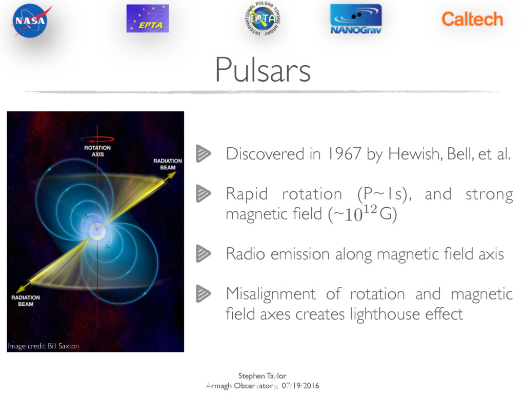
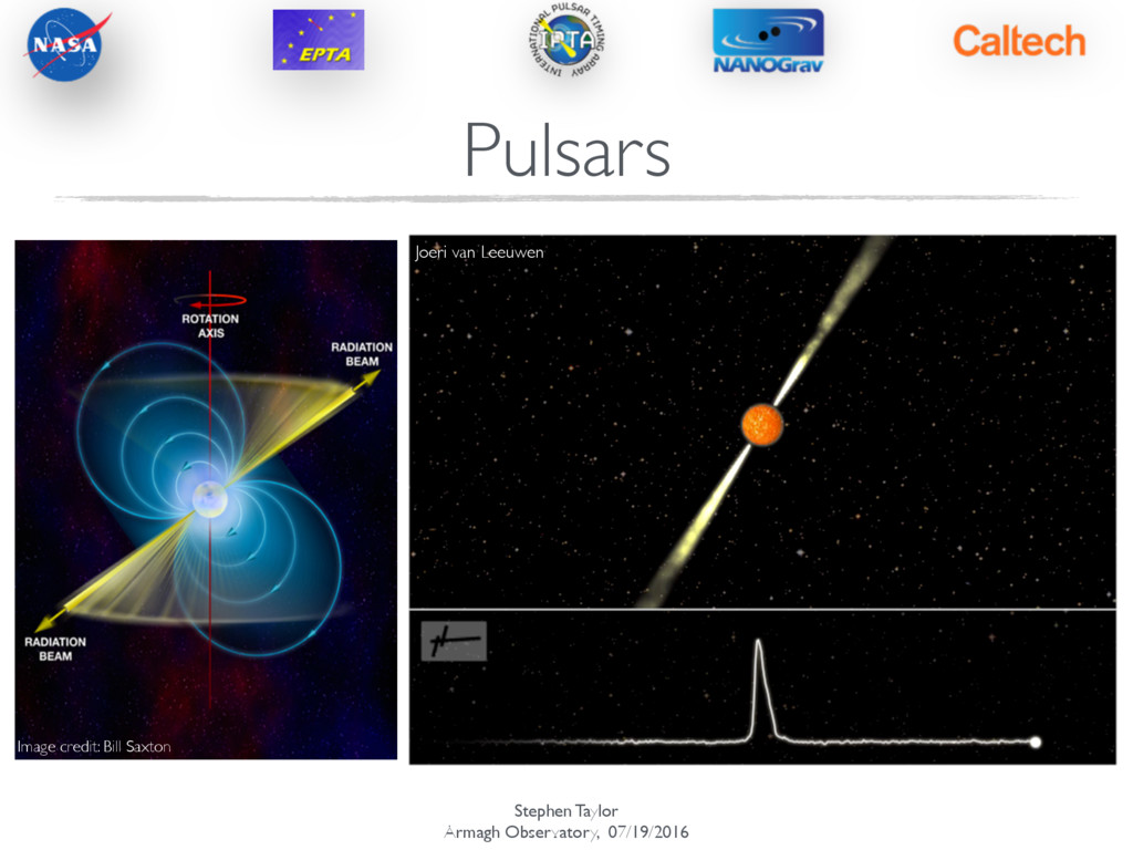
19. Stephen Taylor Armagh Observatory, 07/19/2016 Discovered in 1967 by Hewish, Bell, et al. ! Rapid rotation (P~1s), and strong magnetic field (~ G) ! Radio emission along magnetic field axis ! Misalignment of rotation and magnetic field axes creates lighthouse effect 1012 Image credit: Bill Saxton Pulsars
20. Stephen Taylor Armagh Observatory, 07/19/2016 Discovered in 1967 by Hewish, Bell, et al. ! Rapid rotation (P~1s), and strong magnetic field (~ G) ! Radio emission along magnetic field axis ! Misalignment of rotation and magnetic field axes creates lighthouse effect 1012 Image credit: Bill Saxton Joeri van Leeuwen Pulsars
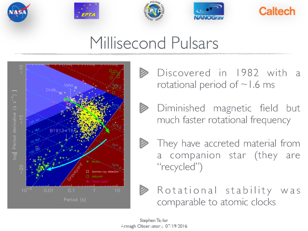
21. Stephen Taylor Armagh Observatory, 07/19/2016 Millisecond Pulsars Discovered in 1982 with a rotational period of ~1.6 ms ! Diminished magnetic field but much faster rotational frequency ! They have accreted material from a companion star (they are “recycled”) ! R o t a t i o n a l s t a b i l i t y w a s comparable to atomic clocks
22. Stephen Taylor Armagh Observatory, 07/19/2016 Pulsar timing ! Sophisticated timing models depend on P, Pdot, pulsar sky location, ISM properties, pulsar binary parameters etc….. Image credit: Duncan Lorimer
23. Stephen Taylor Armagh Observatory, 07/19/2016 good timing-solution error in frequency derivative error in position unmodeled proper motion Lorimer & Kramer (2005)
24. Stephen Taylor Armagh Observatory, 07/19/2016
25. Stephen Taylor Armagh Observatory, 07/19/2016 John Rowe Animation/Australia Telescope National Facility, CSIRO
26. Stephen Taylor Armagh Observatory, 07/19/2016
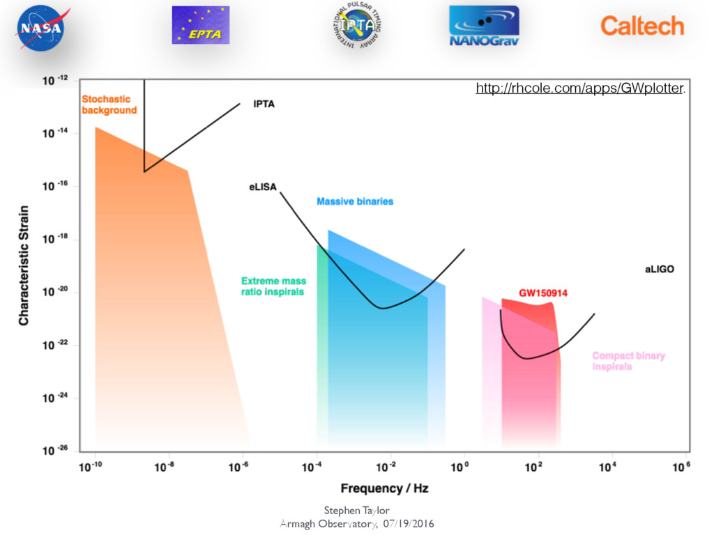
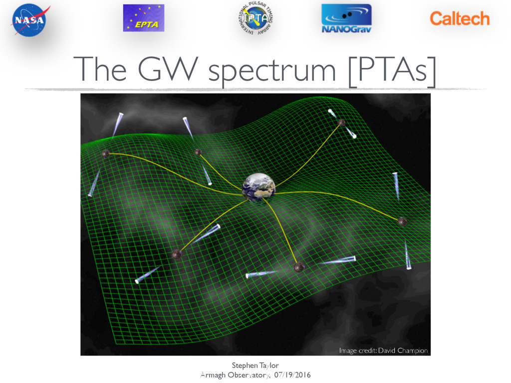
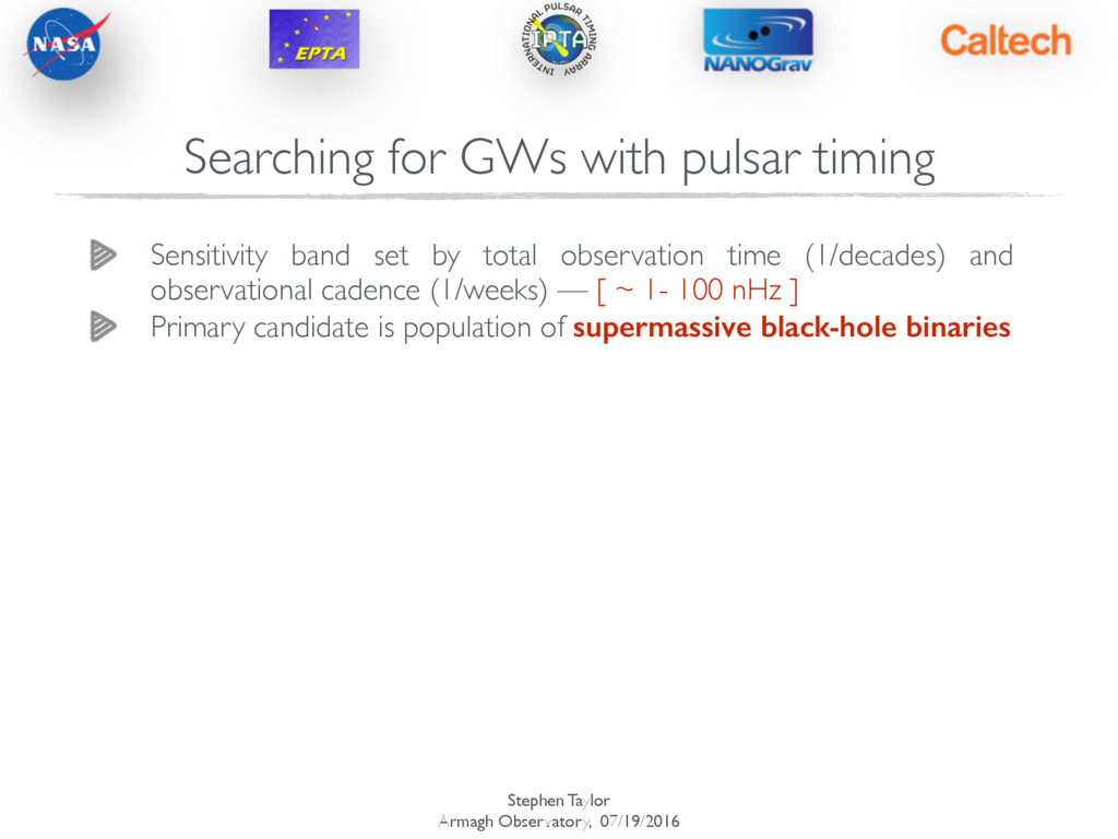
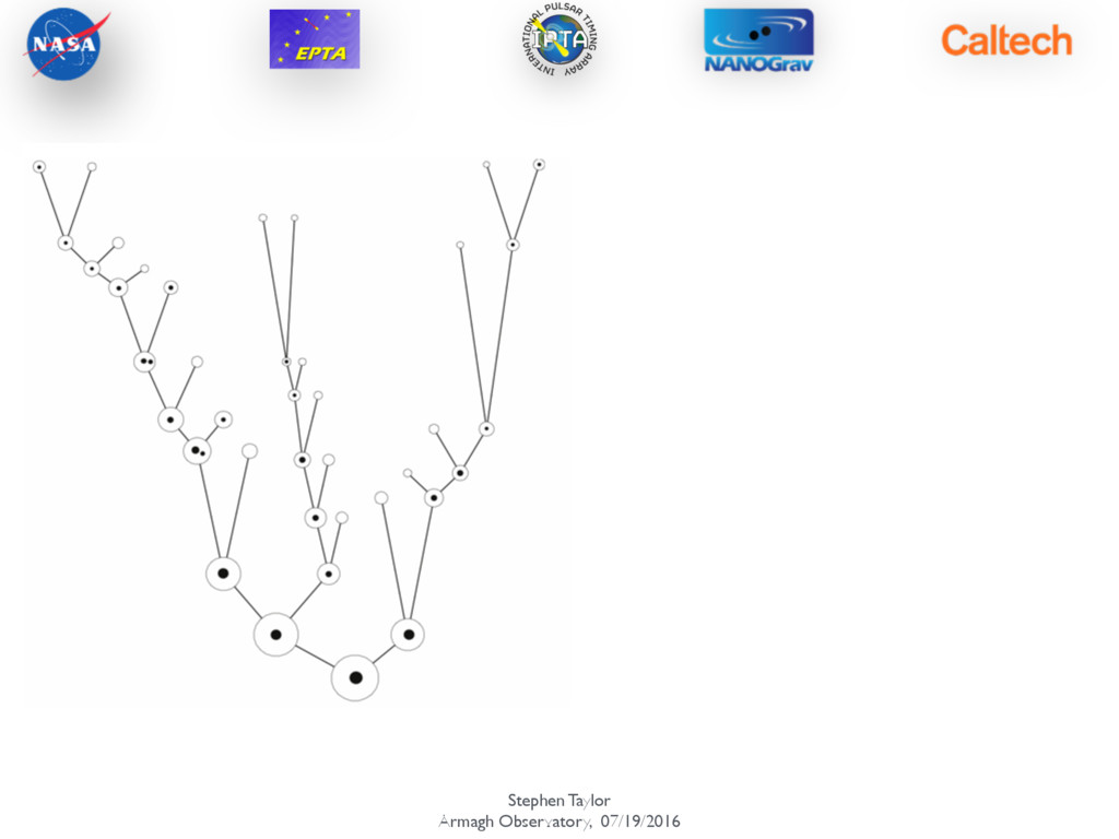
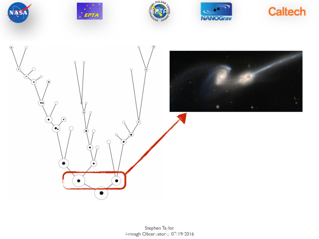
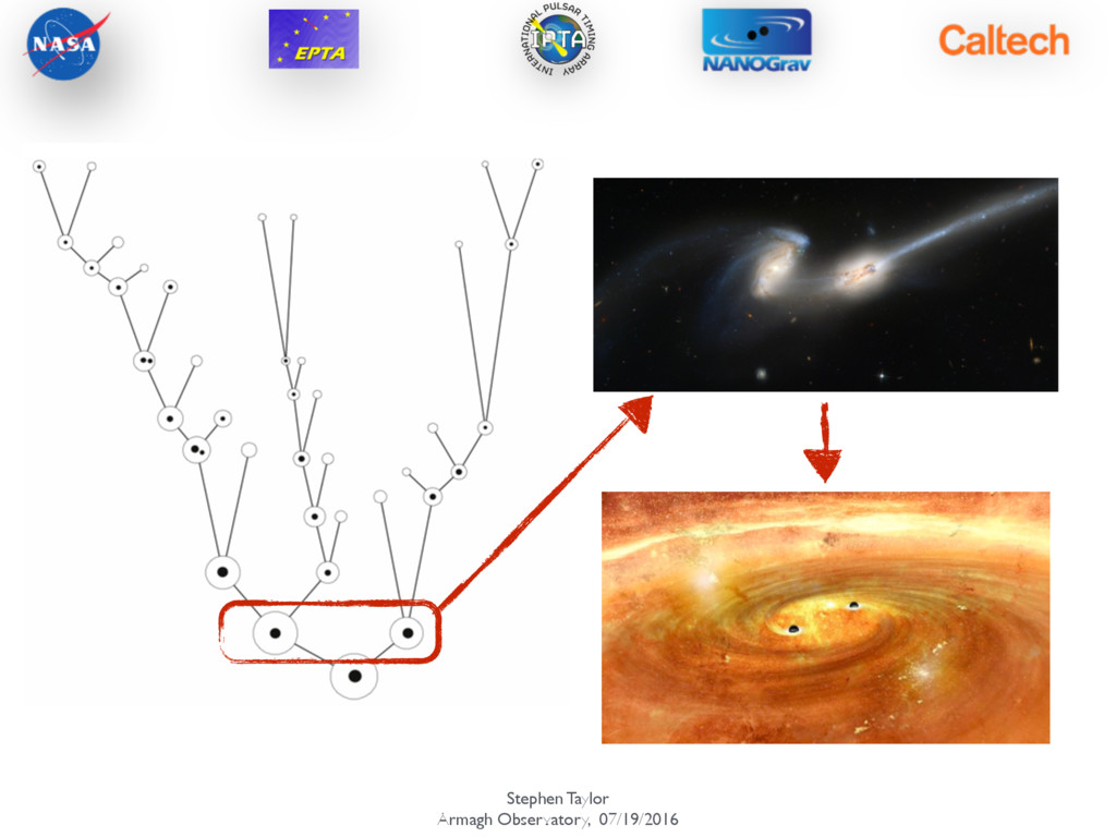
27. Stephen Taylor Armagh Observatory, 07/19/2016 Sensitivity band set by total observation time (1/decades) and observational cadence (1/weeks) — [ ~ 1- 100 nHz ] Primary candidate is population of supermassive black-hole binaries Searching for GWs with pulsar timing
28. Stephen Taylor Armagh Observatory, 07/19/2016 Sensitivity band set by total observation time (1/decades) and observational cadence (1/weeks) — [ ~ 1- 100 nHz ] Primary candidate is population of supermassive black-hole binaries Image credit: CSIRO Searching for GWs with pulsar timing
29. Stephen Taylor Armagh Observatory, 07/19/2016 Sensitivity band set by total observation time (1/decades) and observational cadence (1/weeks) — [ ~ 1- 100 nHz ] Primary candidate is population of supermassive black-hole binaries Image credit: CSIRO Searching for GWs with pulsar timing
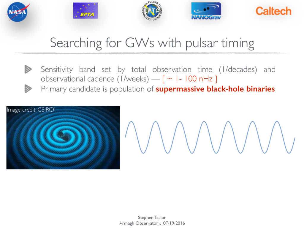
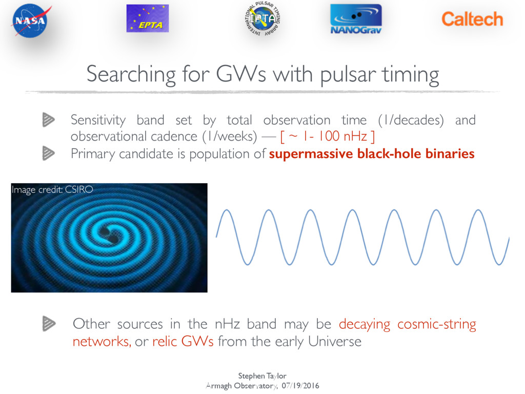
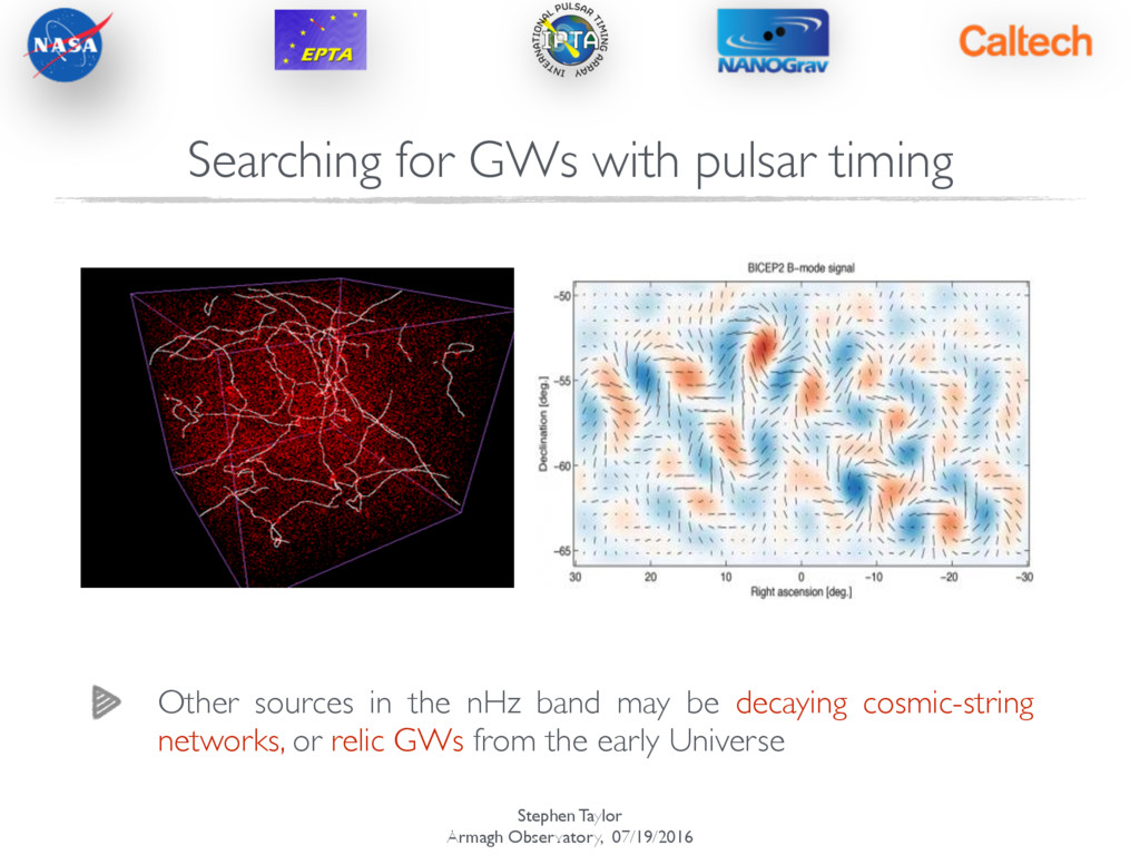
30. Stephen Taylor Armagh Observatory, 07/19/2016 Sensitivity band set by total observation time (1/decades) and observational cadence (1/weeks) — [ ~ 1- 100 nHz ] Primary candidate is population of supermassive black-hole binaries Image credit: CSIRO Searching for GWs with pulsar timing Other sources in the nHz band may be decaying cosmic-string networks, or relic GWs from the early Universe
31. Stephen Taylor Armagh Observatory, 07/19/2016 Other sources in the nHz band may be decaying cosmic-string networks, or relic GWs from the early Universe Searching for GWs with pulsar timing
32. Stephen Taylor Armagh Observatory, 07/19/2016 Image credit: David Champion
33. Stephen Taylor Armagh Observatory, 07/19/2016 Image credit: David Champion Hellings & Downs (1983)
34. Stephen Taylor Armagh Observatory, 07/19/2016 0 20 40 60 80 100 120 140 160 180 pulsar angular separation [deg] -0.2 0.0 0.2 0.4 0.6 0.8 1.0 arrival time correlation N = 1 Npairs = N(N 1)/2 Assessing detection significance
35. Stephen Taylor Armagh Observatory, 07/19/2016 0 20 40 60 80 100 120 140 160 180 pulsar angular separation [deg] -0.2 0.0 0.2 0.4 0.6 0.8 1.0 arrival time correlation N = 1 0 20 40 60 80 100 120 140 160 180 pulsar angular separation [deg] -0.2 0.0 0.2 0.4 0.6 0.8 1.0 arrival time correlation N = 4 Npairs = N(N 1)/2 Assessing detection significance
36. Stephen Taylor Armagh Observatory, 07/19/2016 0 20 40 60 80 100 120 140 160 180 pulsar angular separation [deg] -0.2 0.0 0.2 0.4 0.6 0.8 1.0 arrival time correlation N = 1 0 20 40 60 80 100 120 140 160 180 pulsar angular separation [deg] -0.2 0.0 0.2 0.4 0.6 0.8 1.0 arrival time correlation N = 4 0 20 40 60 80 100 120 140 160 180 pulsar angular separation [deg] -0.2 0.0 0.2 0.4 0.6 0.8 1.0 arrival time correlation N = 10 Npairs = N(N 1)/2 Assessing detection significance
37. Stephen Taylor Armagh Observatory, 07/19/2016 0 20 40 60 80 100 120 140 160 180 pulsar angular separation [deg] -0.2 0.0 0.2 0.4 0.6 0.8 1.0 arrival time correlation N = 1 0 20 40 60 80 100 120 140 160 180 pulsar angular separation [deg] -0.2 0.0 0.2 0.4 0.6 0.8 1.0 arrival time correlation N = 4 0 20 40 60 80 100 120 140 160 180 pulsar angular separation [deg] -0.2 0.0 0.2 0.4 0.6 0.8 1.0 arrival time correlation N = 10 0 20 40 60 80 100 120 140 160 180 pulsar angular separation [deg] -0.2 0.0 0.2 0.4 0.6 0.8 1.0 arrival time correlation N = 30 Npairs = N(N 1)/2 Assessing detection significance
38. Stephen Taylor Armagh Observatory, 07/19/2016 0 20 40 60 80 100 120 140 160 180 pulsar angular separation [deg] -0.2 0.0 0.2 0.4 0.6 0.8 1.0 arrival time correlation N = 1 0 20 40 60 80 100 120 140 160 180 pulsar angular separation [deg] -0.2 0.0 0.2 0.4 0.6 0.8 1.0 arrival time correlation N = 4 0 20 40 60 80 100 120 140 160 180 pulsar angular separation [deg] -0.2 0.0 0.2 0.4 0.6 0.8 1.0 arrival time correlation N = 10 0 20 40 60 80 100 120 140 160 180 pulsar angular separation [deg] -0.2 0.0 0.2 0.4 0.6 0.8 1.0 arrival time correlation N = 30 0 20 40 60 80 100 120 140 160 180 pulsar angular separation [deg] -0.2 0.0 0.2 0.4 0.6 0.8 1.0 arrival time correlation N = 50 Npairs = N(N 1)/2 Assessing detection significance
39. Stephen Taylor Armagh Observatory, 07/19/2016 0 5 10 PPTA4 0 20 40 60 80 100 NANOGrav+ 0 20 40 60 80 100 EPTA+ 0 20 40 60 80 100 IPTA+ 0 5 10 15 20 T [yrs] 0 20 40 60 80 100 TPTA Expected detection probability [%] Taylor et al. (2016a), ApJL 819, L6
40. Stephen Taylor Armagh Observatory, 07/19/2016
41. Stephen Taylor Armagh Observatory, 07/19/2016
42. Stephen Taylor Armagh Observatory, 07/19/2016
43. Stephen Taylor Armagh Observatory, 07/19/2016 “Final parsec problem” Dynamical friction not a sufficient driving mechanism to induce merger within a Hubble time e.g., Milosavljevic & Merritt (2003) Searching for GWs with pulsar timing
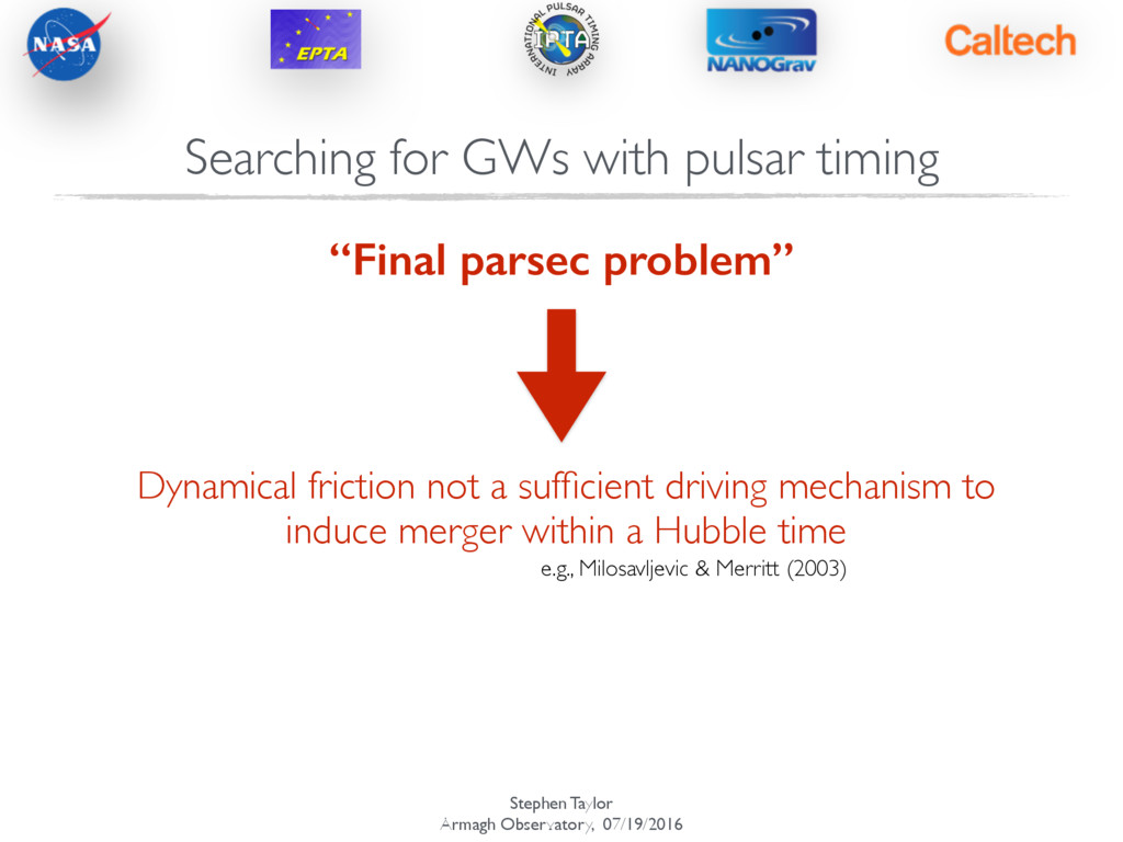
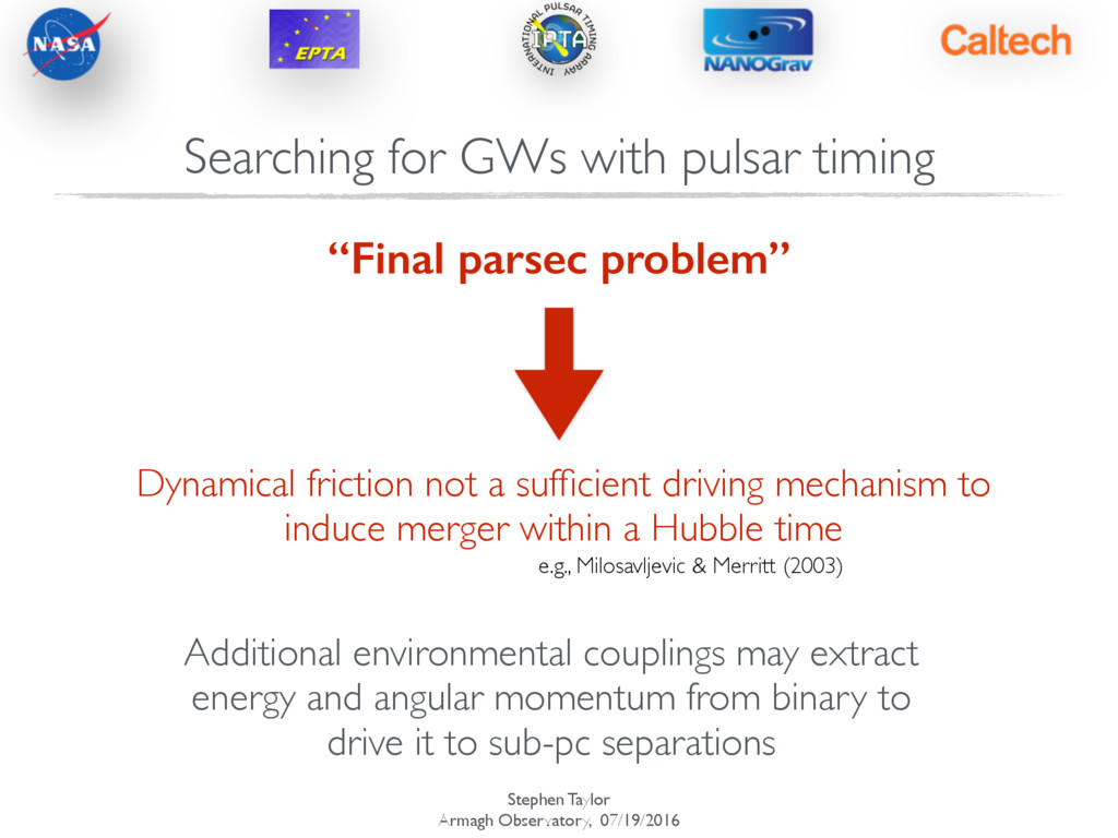
44. Stephen Taylor Armagh Observatory, 07/19/2016 “Final parsec problem” Dynamical friction not a sufficient driving mechanism to induce merger within a Hubble time e.g., Milosavljevic & Merritt (2003) Additional environmental couplings may extract energy and angular momentum from binary to drive it to sub-pc separations Searching for GWs with pulsar timing
45. Stephen Taylor Armagh Observatory, 07/19/2016
46. Stephen Taylor Armagh Observatory, 07/19/2016 circumbinary disk interaction stellar hardening binary eccentricity
47. Stephen Taylor Armagh Observatory, 07/19/2016 circumbinary disk interaction stellar hardening binary eccentricity 10-9 10-8 10-7 f [Hz] 10-15 10-14 hc(f) hc(f = 1yr-1) = A = 1⇥10-15 T = 9 yrs
48. Stephen Taylor Armagh Observatory, 07/19/2016 circumbinary disk interaction stellar hardening binary eccentricity 10-9 10-8 10-7 f [Hz] 10-15 10-14 hc(f) hc(f = 1yr-1) = A = 1⇥10-15 T = 9 yrs 10-9 10-8 10-7 f [Hz] 10-15 10-14 hc(f) hc(f = 1yr-1) = A = 1⇥10-15 T = 11 yrs
49. Stephen Taylor Armagh Observatory, 07/19/2016 circumbinary disk interaction stellar hardening binary eccentricity 10-9 10-8 10-7 f [Hz] 10-15 10-14 hc(f) hc(f = 1yr-1) = A = 1⇥10-15 T = 9 yrs 10-9 10-8 10-7 f [Hz] 10-15 10-14 hc(f) hc(f = 1yr-1) = A = 1⇥10-15 T = 11 yrs 10-9 10-8 10-7 f [Hz] 10-15 10-14 hc(f) hc(f = 1yr-1) = A = 1⇥10-15 T = 15 yrs
50. Stephen Taylor Armagh Observatory, 07/19/2016 circumbinary disk interaction stellar hardening binary eccentricity 10-9 10-8 10-7 f [Hz] 10-15 10-14 hc(f) hc(f = 1yr-1) = A = 1⇥10-15 T = 9 yrs 10-9 10-8 10-7 f [Hz] 10-15 10-14 hc(f) hc(f = 1yr-1) = A = 1⇥10-15 T = 11 yrs 10-9 10-8 10-7 f [Hz] 10-15 10-14 hc(f) hc(f = 1yr-1) = A = 1⇥10-15 T = 15 yrs 10-9 10-8 10-7 f [Hz] 10-15 10-14 hc(f) hc(f = 1yr-1) = A = 1⇥10-15 T = 30 yrs
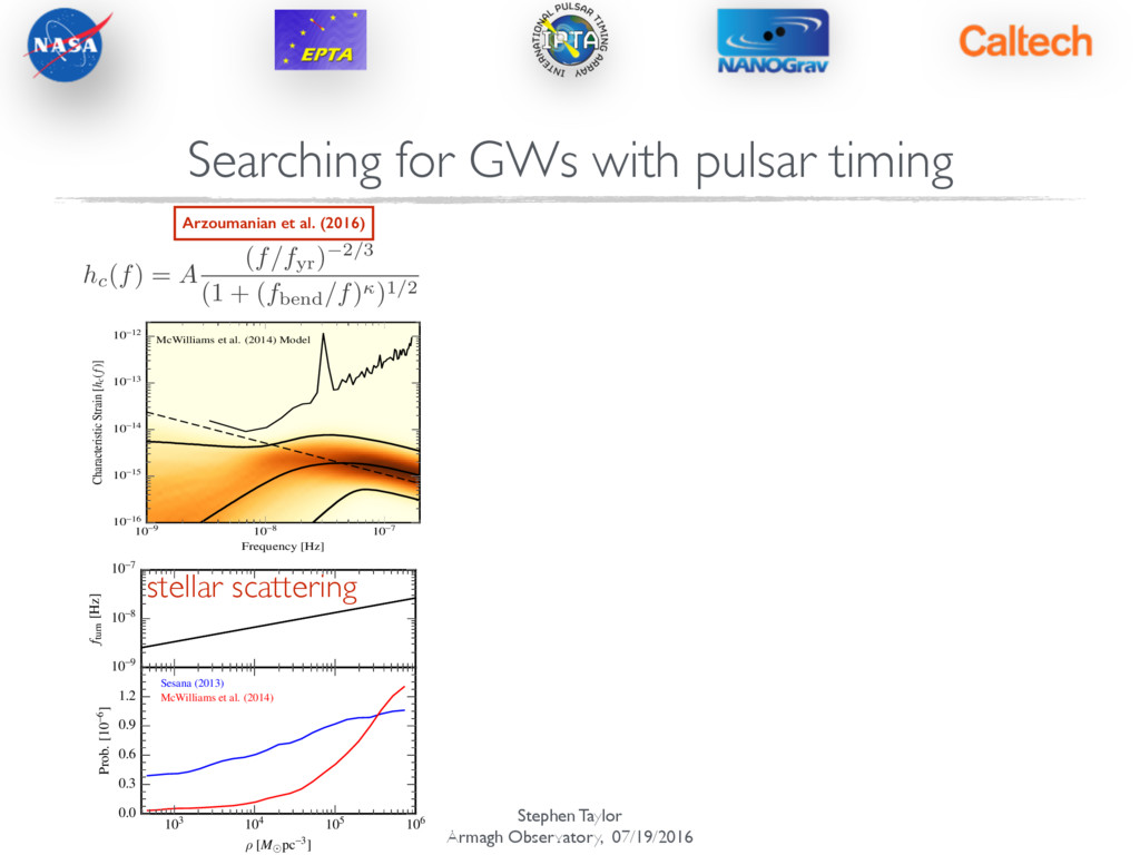
51. Stephen Taylor Armagh Observatory, 07/19/2016 12 10-9 10-8 10-7 Frequency [Hz] 10-16 10-15 10-14 10-13 10-12 Characteristic Strain [hc(f)] McWilliams et al. (2014) Model Figure 5. Probability density plots of the recovered GWB spectra for models A and B using the broken-power-law model parameterized by (Agw, fbend, and ) as discussed in the text. The thick black lines indicate the 95% credible region and median of the GWB spectrum. The dashed line shows the 95% upper limit on the amplitude of purely GW-driven spectrum using the Gaussian priors on the amplitude from models A and B, respectively. The thin black curve shows the 95% upper limit on the GWB spectrum from the spectral analysis. 16 10-9 10-8 10-7 fturn [Hz] 103 104 105 106 ⇢ [M pc-3] 0.0 0.3 0.6 0.9 1.2 Prob. [10-6] Sesana (2013) McWilliams et al. (2014) stellar scattering hc(f) = A (f/fyr) 2/3 (1 + (fbend/f))1/2 Arzoumanian et al. (2016) Searching for GWs with pulsar timing
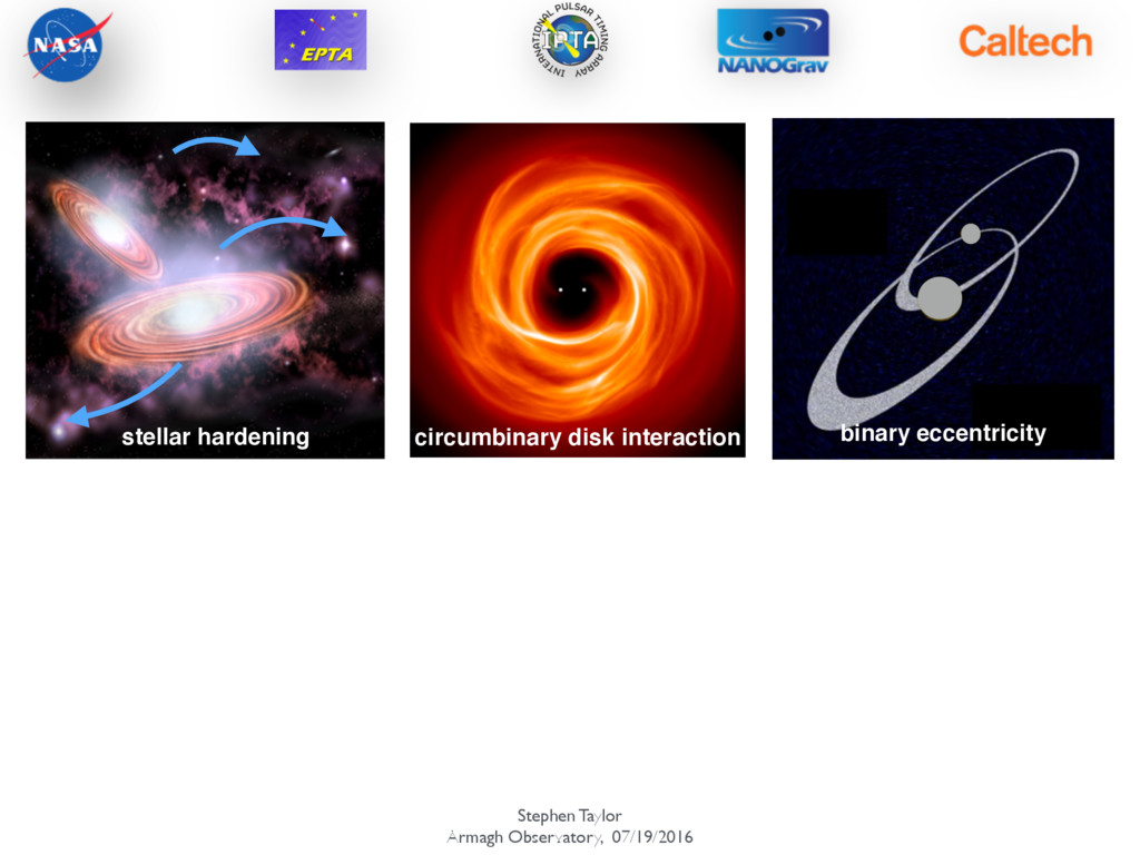
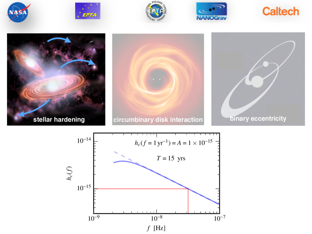
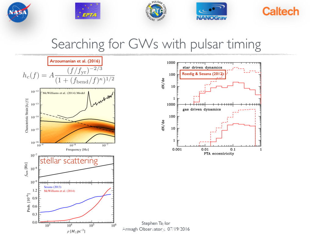
52. Stephen Taylor Armagh Observatory, 07/19/2016 12 10-9 10-8 10-7 Frequency [Hz] 10-16 10-15 10-14 10-13 10-12 Characteristic Strain [hc(f)] McWilliams et al. (2014) Model Figure 5. Probability density plots of the recovered GWB spectra for models A and B using the broken-power-law model parameterized by (Agw, fbend, and ) as discussed in the text. The thick black lines indicate the 95% credible region and median of the GWB spectrum. The dashed line shows the 95% upper limit on the amplitude of purely GW-driven spectrum using the Gaussian priors on the amplitude from models A and B, respectively. The thin black curve shows the 95% upper limit on the GWB spectrum from the spectral analysis. 16 10-9 10-8 10-7 fturn [Hz] 103 104 105 106 ⇢ [M pc-3] 0.0 0.3 0.6 0.9 1.2 Prob. [10-6] Sesana (2013) McWilliams et al. (2014) stellar scattering hc(f) = A (f/fyr) 2/3 (1 + (fbend/f))1/2 Figure 2. Eccentricity population of MBHBs detectable by ELISA/NGO and PTAs, expected in stellar and gaseous environments. Left panel: The solid histograms represent the efficient models whereas the dashed histograms are for the inefficient models. Right panel: solid his- tograms include all sources producing timing residuals above 3 ns, dashed histograms include all sources producing residual above 10 ns. mechanism (gas/star) we consider two scenarios (efficient/inefficient), to give an idea of the expected eccentricity range. The models are the following (i) gas-efficient: α = 0.3, ˙ m = 1. The migration timescale is maximized for this high values of the disc parameters, and the decoupling occurs in the very late stage of the MBHB evolution; Roedig & Sesana (2012) Arzoumanian et al. (2016) Searching for GWs with pulsar timing
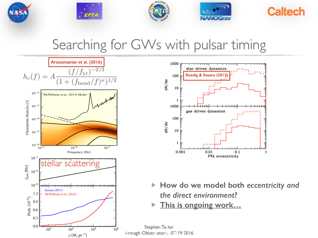
53. Stephen Taylor Armagh Observatory, 07/19/2016 12 10-9 10-8 10-7 Frequency [Hz] 10-16 10-15 10-14 10-13 10-12 Characteristic Strain [hc(f)] McWilliams et al. (2014) Model Figure 5. Probability density plots of the recovered GWB spectra for models A and B using the broken-power-law model parameterized by (Agw, fbend, and ) as discussed in the text. The thick black lines indicate the 95% credible region and median of the GWB spectrum. The dashed line shows the 95% upper limit on the amplitude of purely GW-driven spectrum using the Gaussian priors on the amplitude from models A and B, respectively. The thin black curve shows the 95% upper limit on the GWB spectrum from the spectral analysis. 16 10-9 10-8 10-7 fturn [Hz] 103 104 105 106 ⇢ [M pc-3] 0.0 0.3 0.6 0.9 1.2 Prob. [10-6] Sesana (2013) McWilliams et al. (2014) stellar scattering hc(f) = A (f/fyr) 2/3 (1 + (fbend/f))1/2 Figure 2. Eccentricity population of MBHBs detectable by ELISA/NGO and PTAs, expected in stellar and gaseous environments. Left panel: The solid histograms represent the efficient models whereas the dashed histograms are for the inefficient models. Right panel: solid his- tograms include all sources producing timing residuals above 3 ns, dashed histograms include all sources producing residual above 10 ns. mechanism (gas/star) we consider two scenarios (efficient/inefficient), to give an idea of the expected eccentricity range. The models are the following (i) gas-efficient: α = 0.3, ˙ m = 1. The migration timescale is maximized for this high values of the disc parameters, and the decoupling occurs in the very late stage of the MBHB evolution; Roedig & Sesana (2012) Arzoumanian et al. (2016) How do we model both eccentricity and the direct environment? This is ongoing work… Searching for GWs with pulsar timing
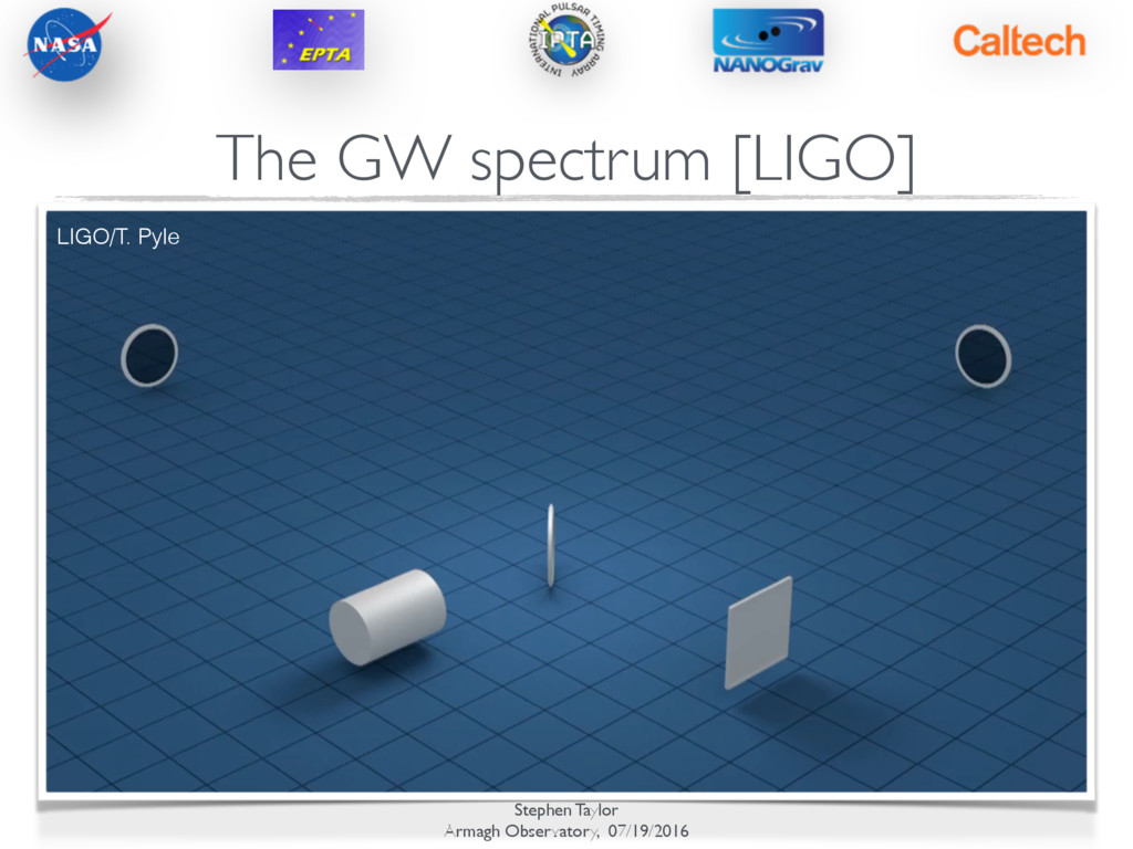
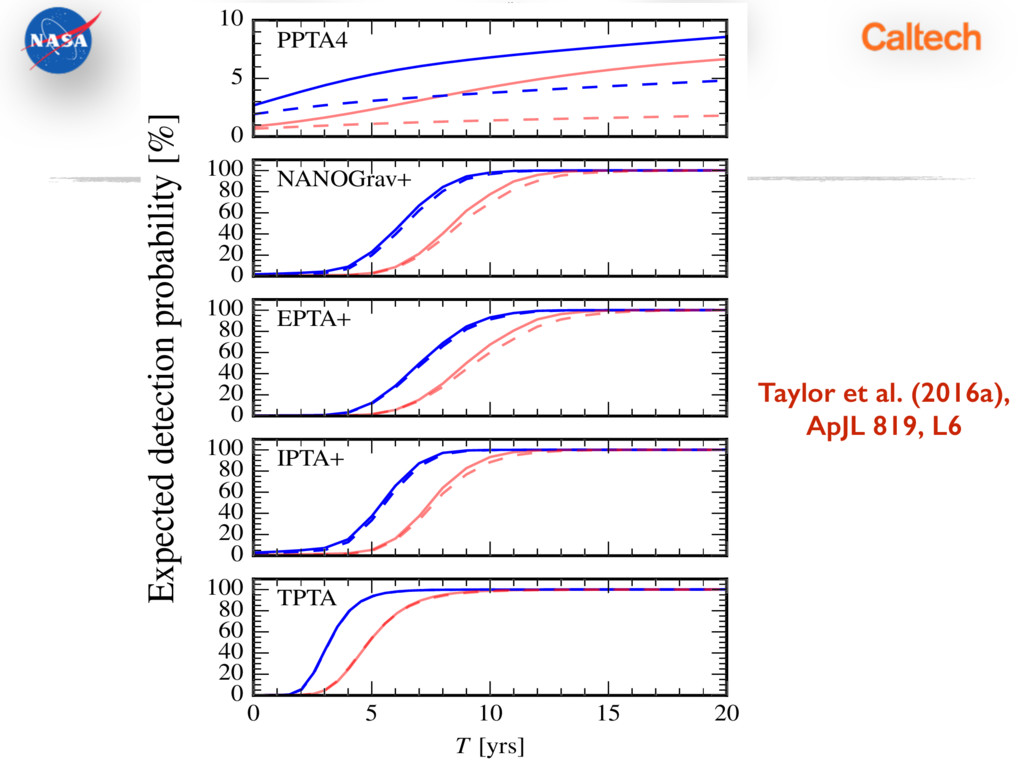
54. Stephen Taylor Armagh Observatory, 07/19/2016 Summary Gravitational-waves have been detected by LIGO. ! (e)LISA will be sensitive to different sources than LIGO. ! PTAs are sensitive to the most massive compact objects in the Universe. ! PTAs are poised to make a detection within 10 years, and will shape our understanding of the final stages of SMBH binary evolution.