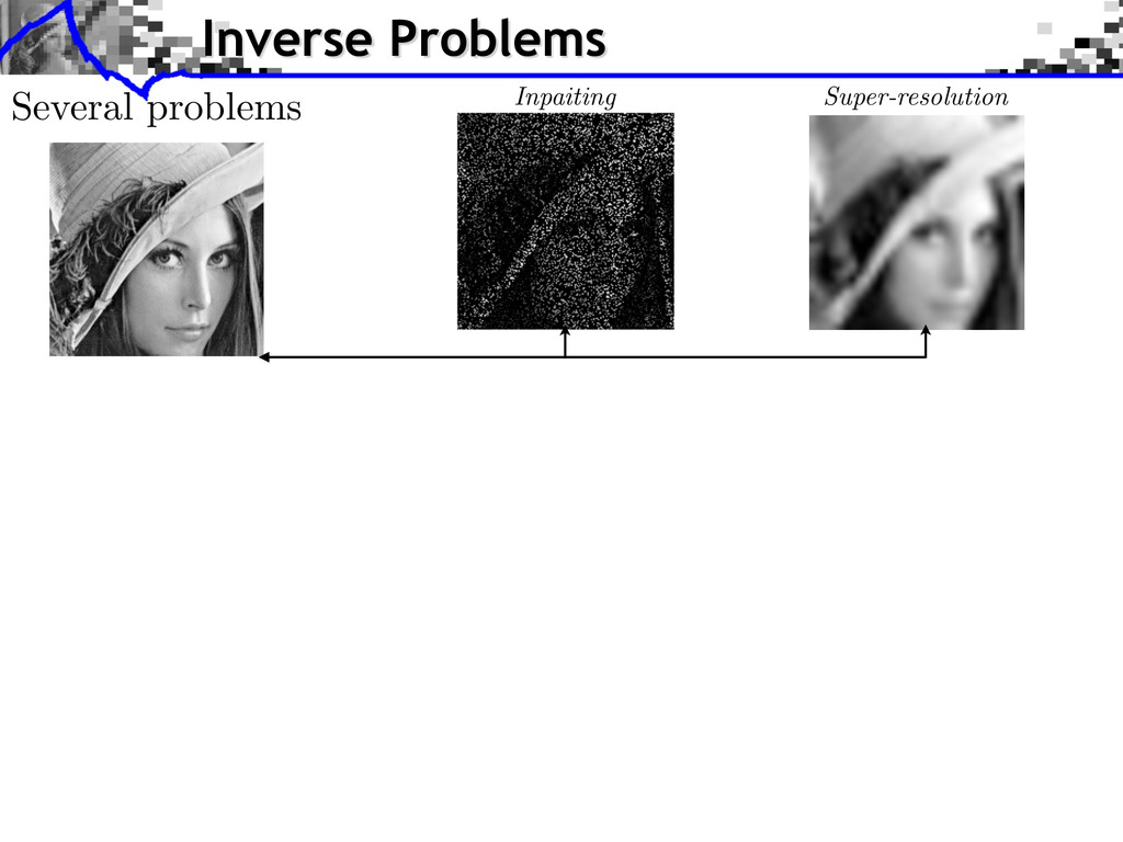
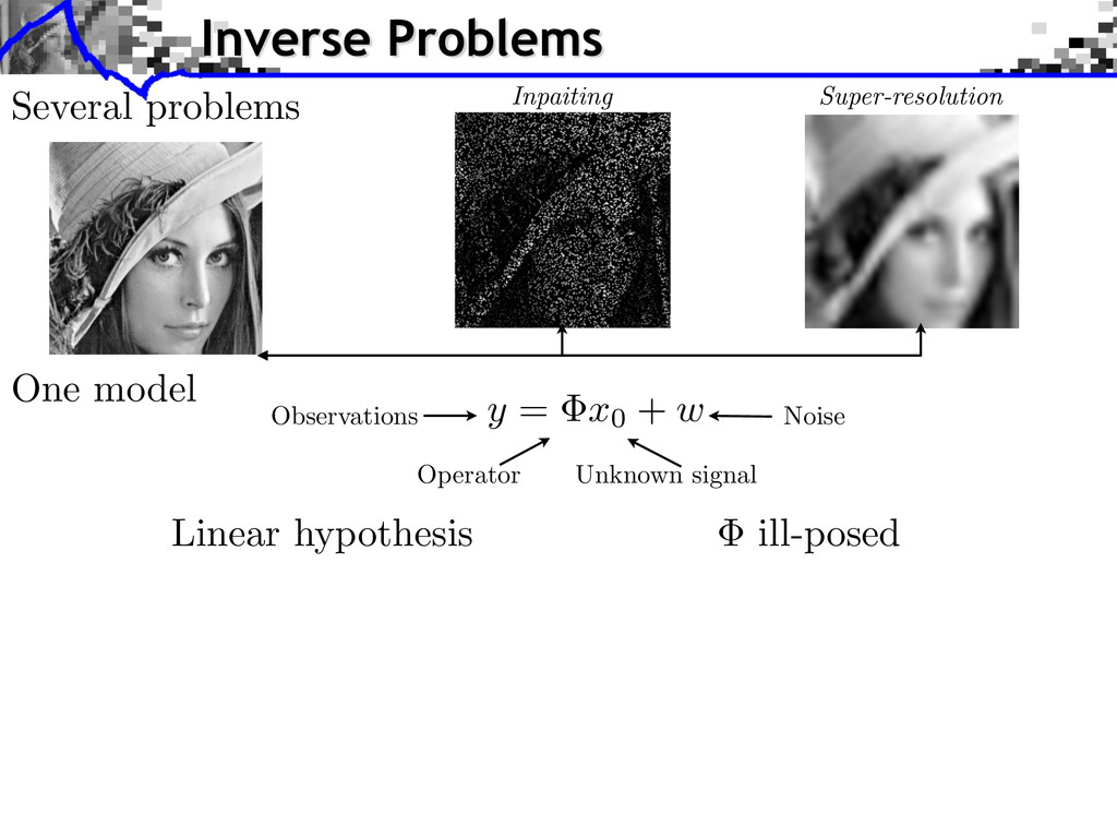
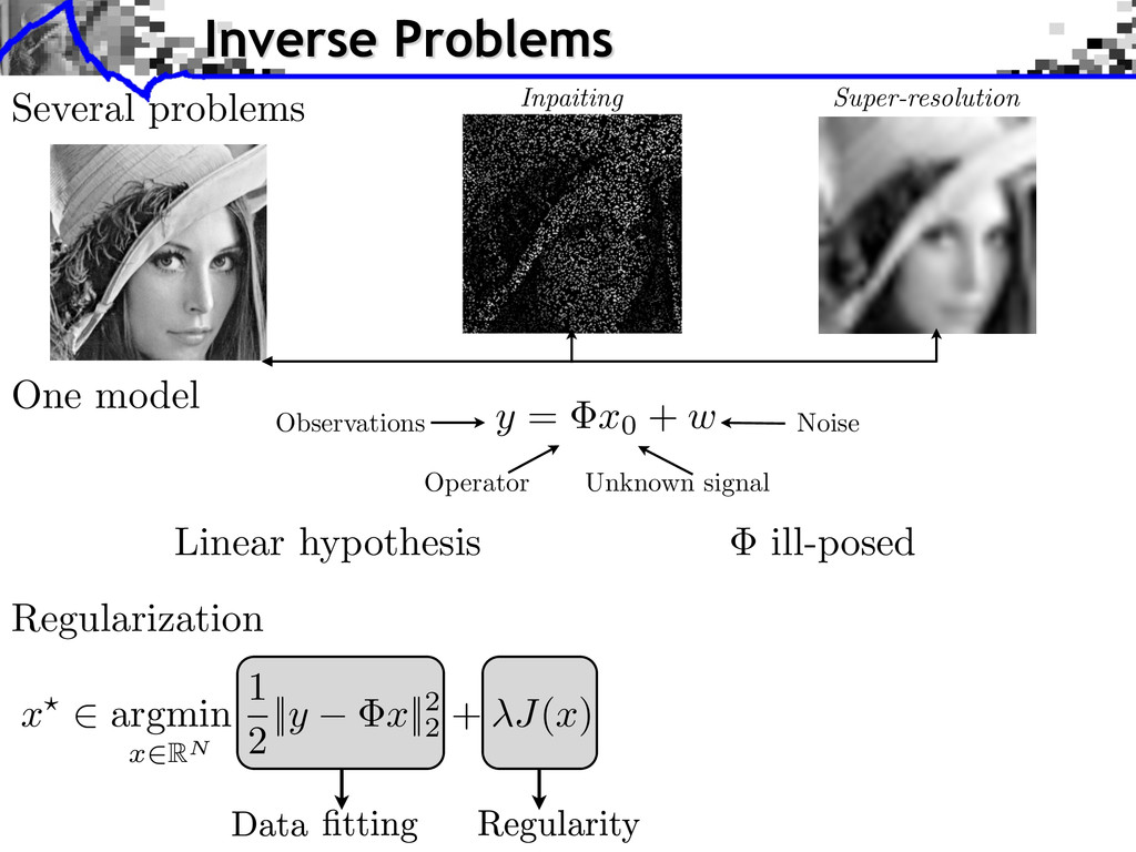
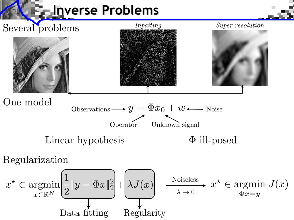
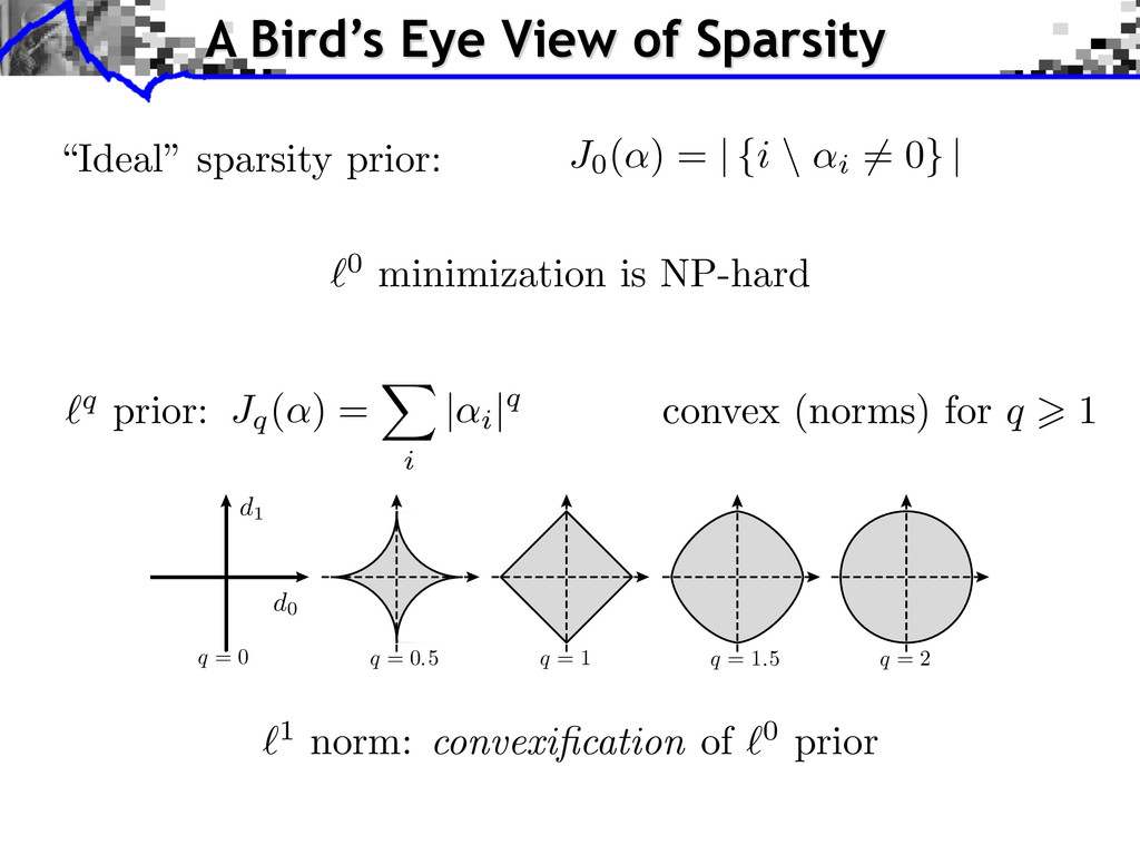
+ w Observations Operator Unknown signal Noise x? 2 argmin x = y J ( x ) Noiseless 0 Several problems Inpaiting Super-resolution Regularization x? 2 argmin x 2RN 1 2 || y x ||2 2 + J ( x )
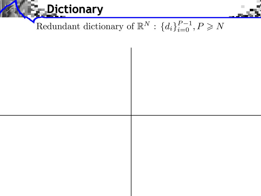
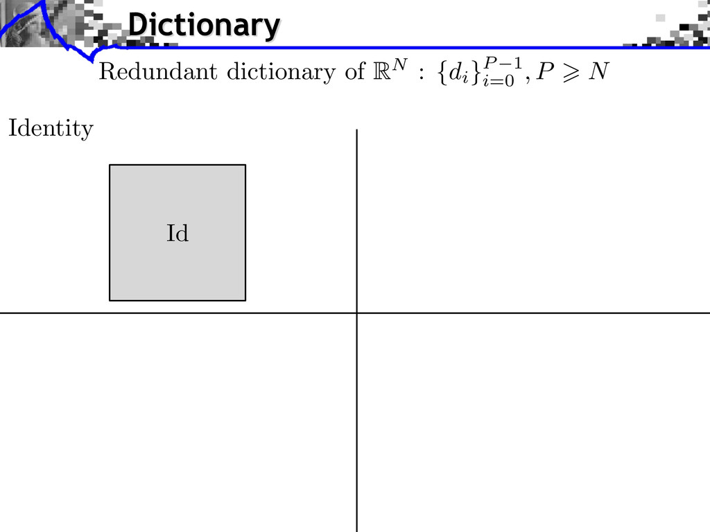
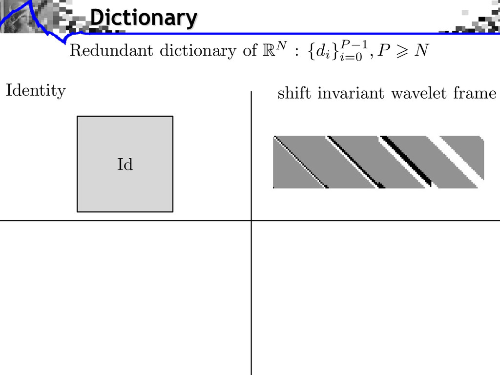
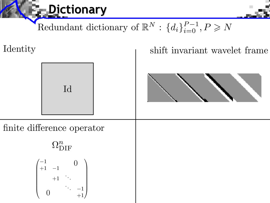
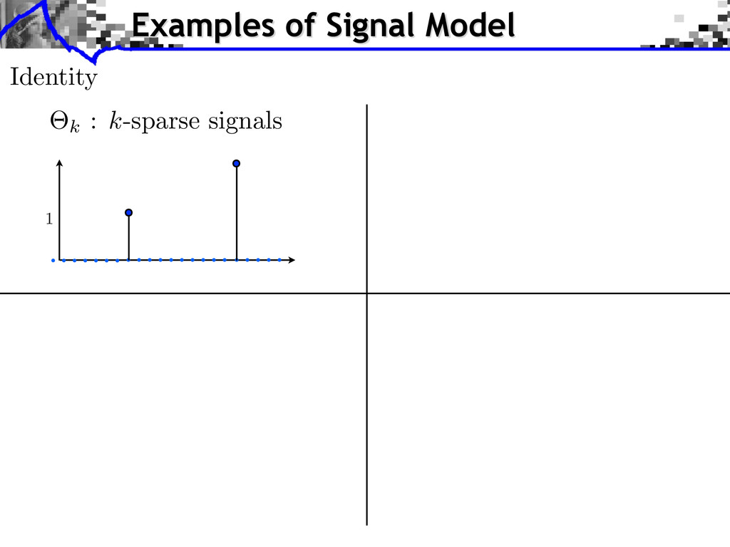
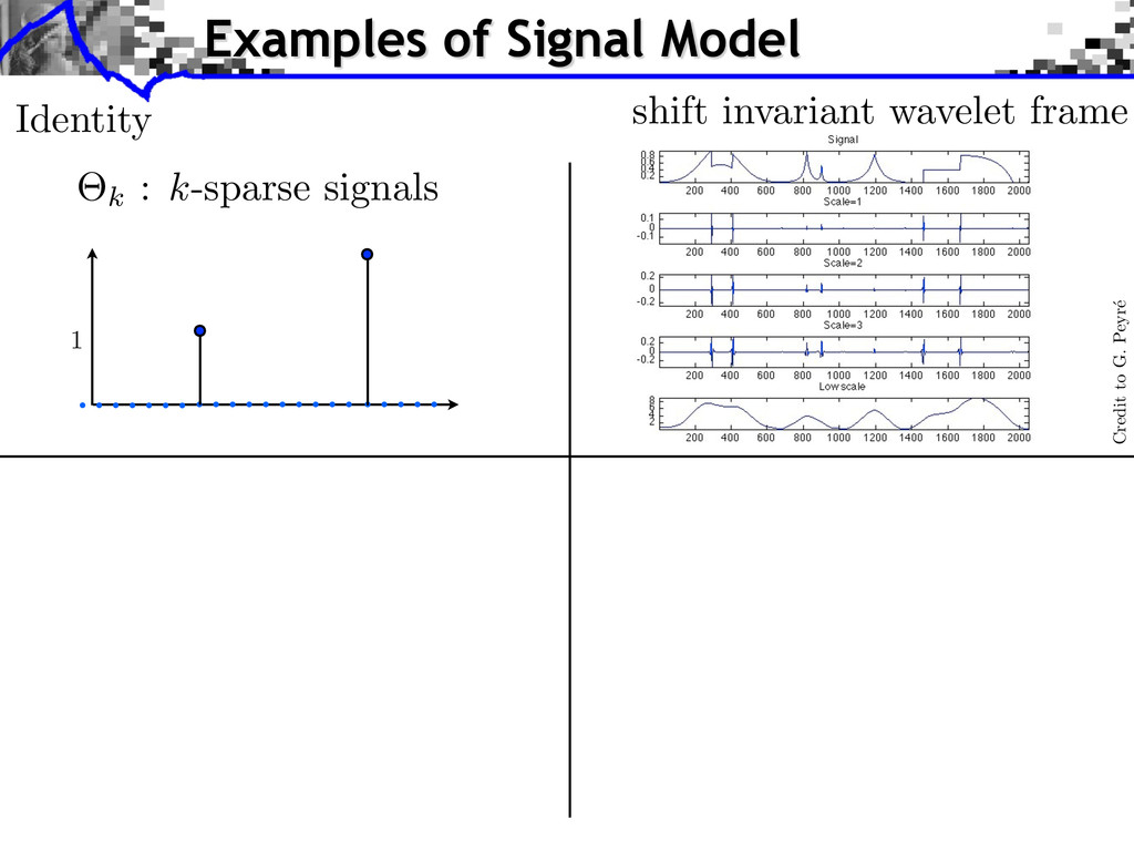
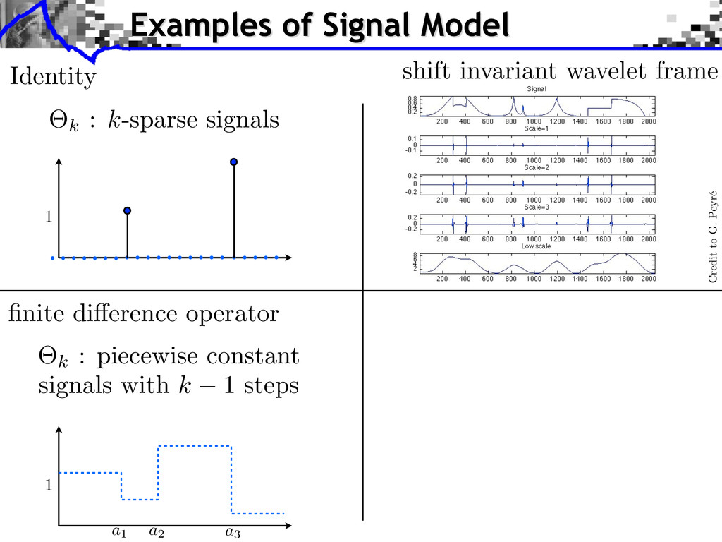
B B @ 1 0 +1 1 +1 ... ... 1 0 +1 1 C C C C C C A Dictionary Redundant dictionary of RN : {di }P 1 i=0 , P > N Identity Id shift invariant wavelet frame
B B @ 1 0 +1 1 +1 ... ... 1 0 +1 1 C C C C C C A Dictionary Redundant dictionary of RN : {di }P 1 i=0 , P > N Identity Id shift invariant wavelet frame fussed lasso ⌦DIF "Id
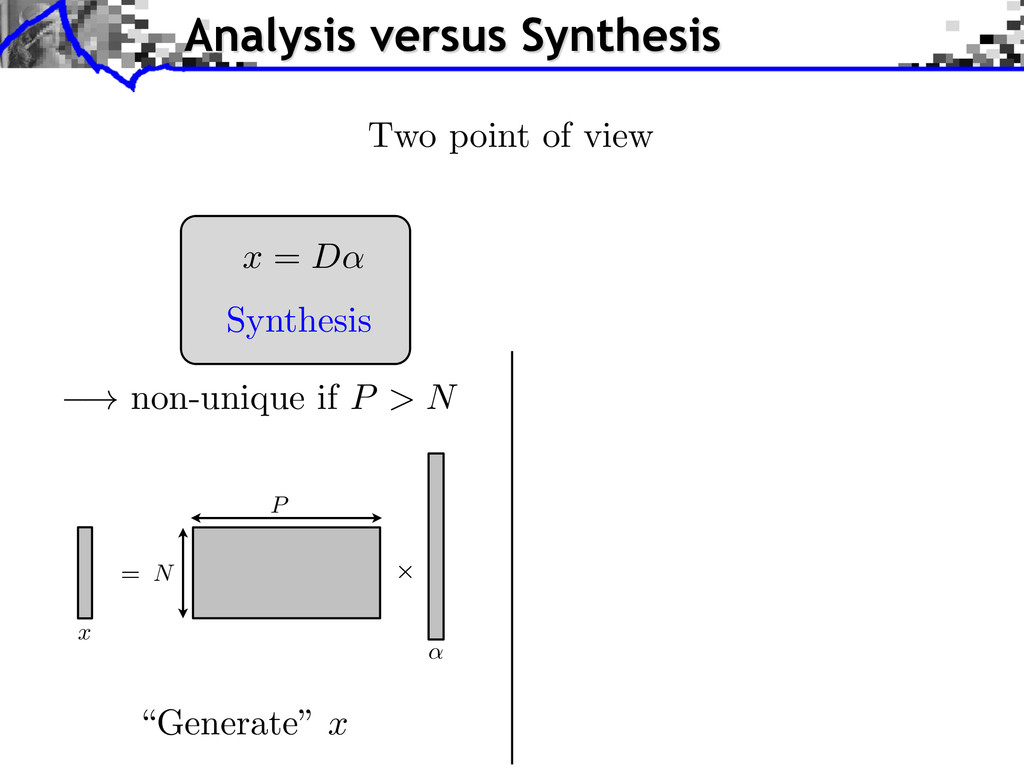
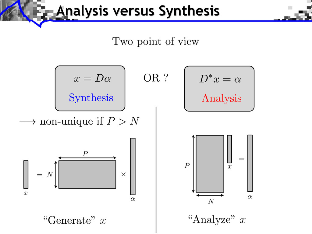
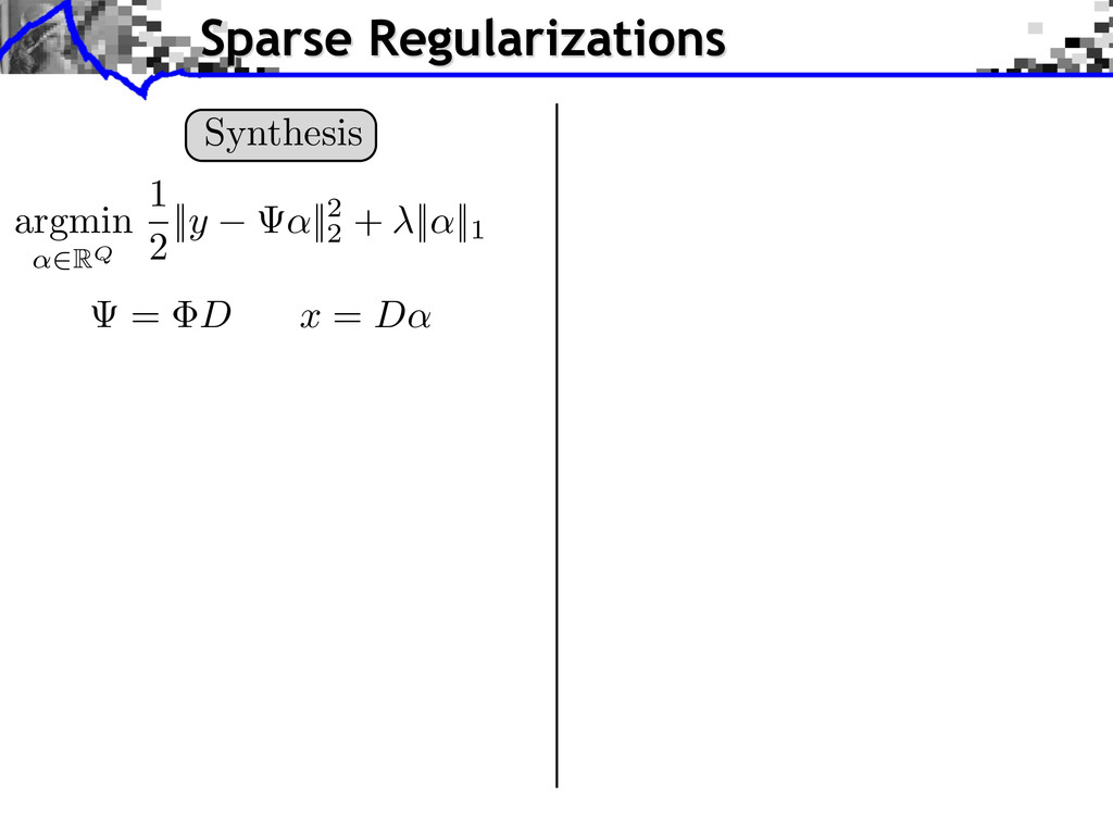
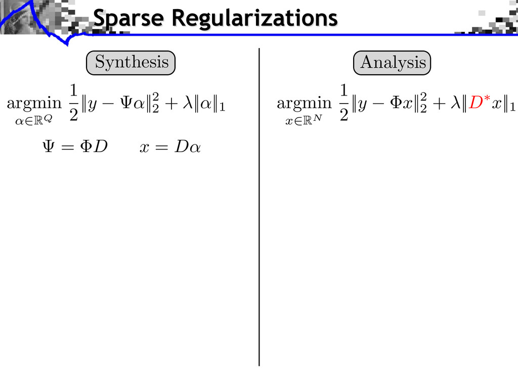
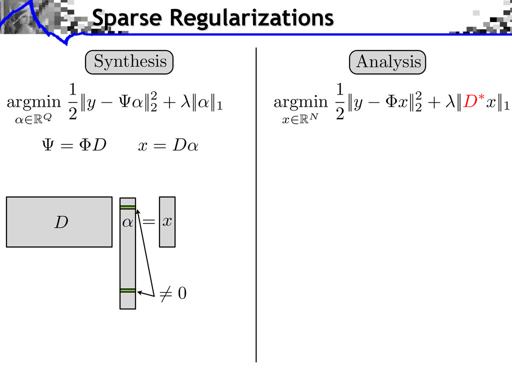
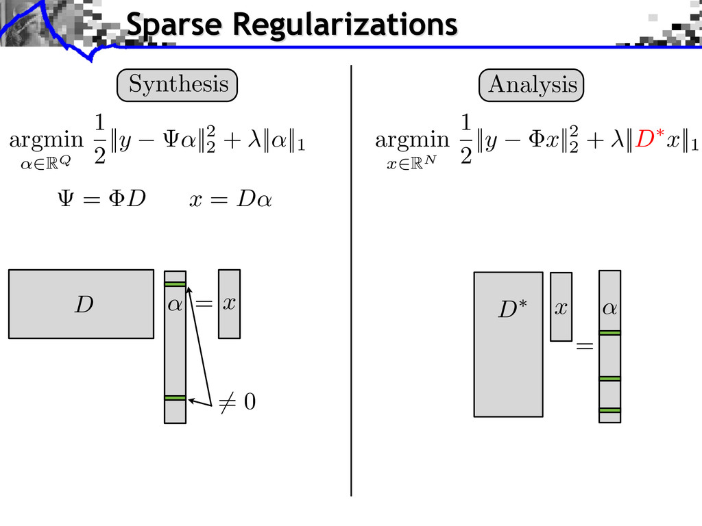
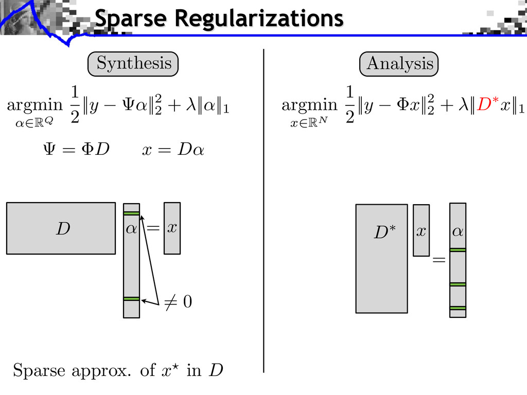
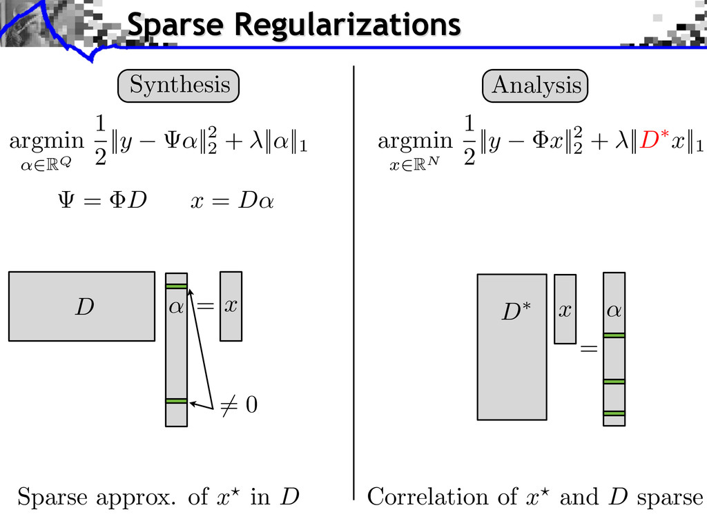
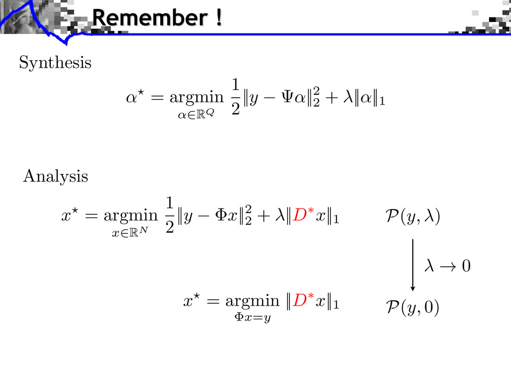
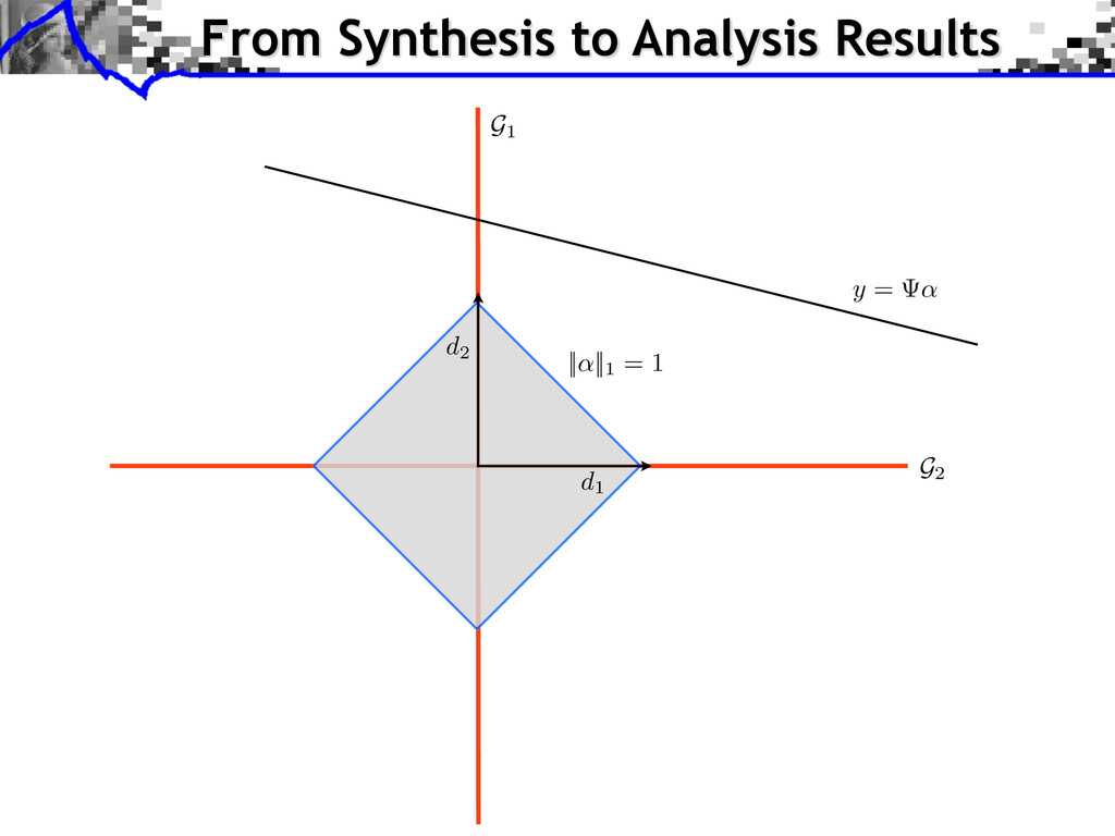
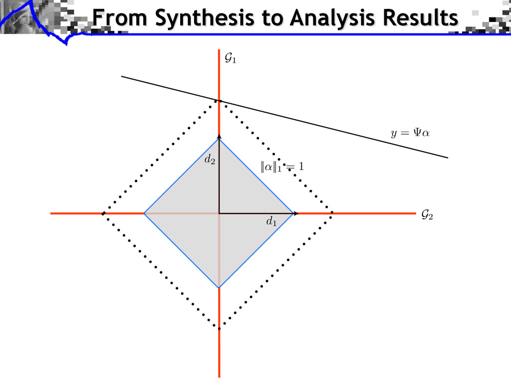
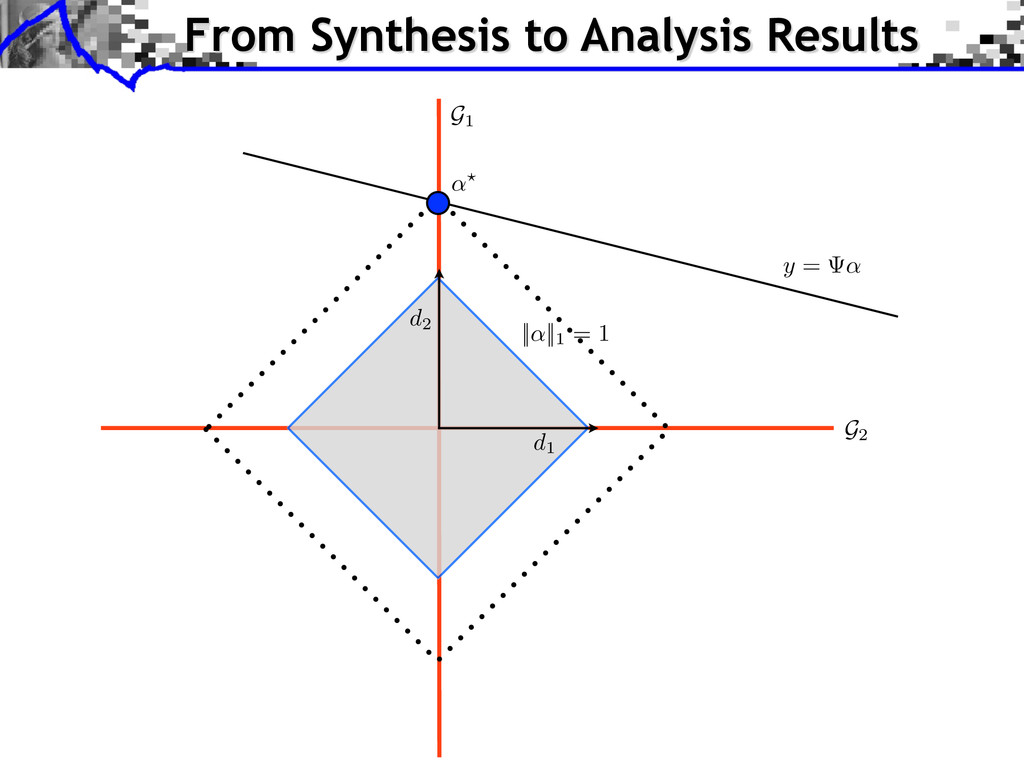
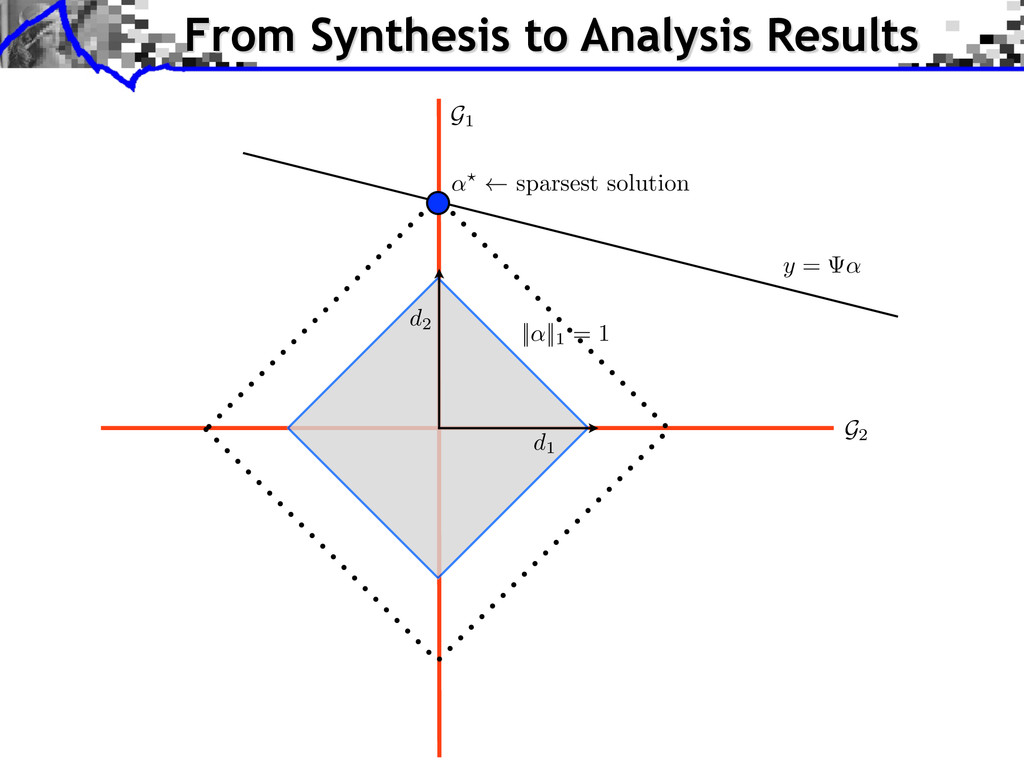
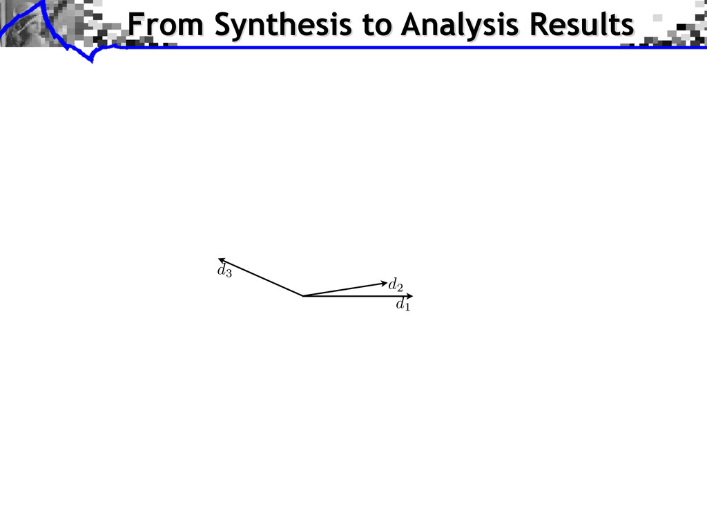
2 + || D ⇤ x ||1 Correlation of x ? and D sparse Sparse approx. of x ? in D Synthesis argmin ↵2RQ 1 2 ||y ↵||2 2 + ||↵||1 = D x = D↵ Sparse Regularizations = 6= 0 D x ↵ = D⇤ x ↵
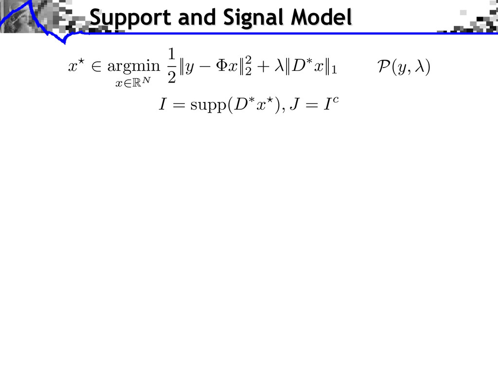
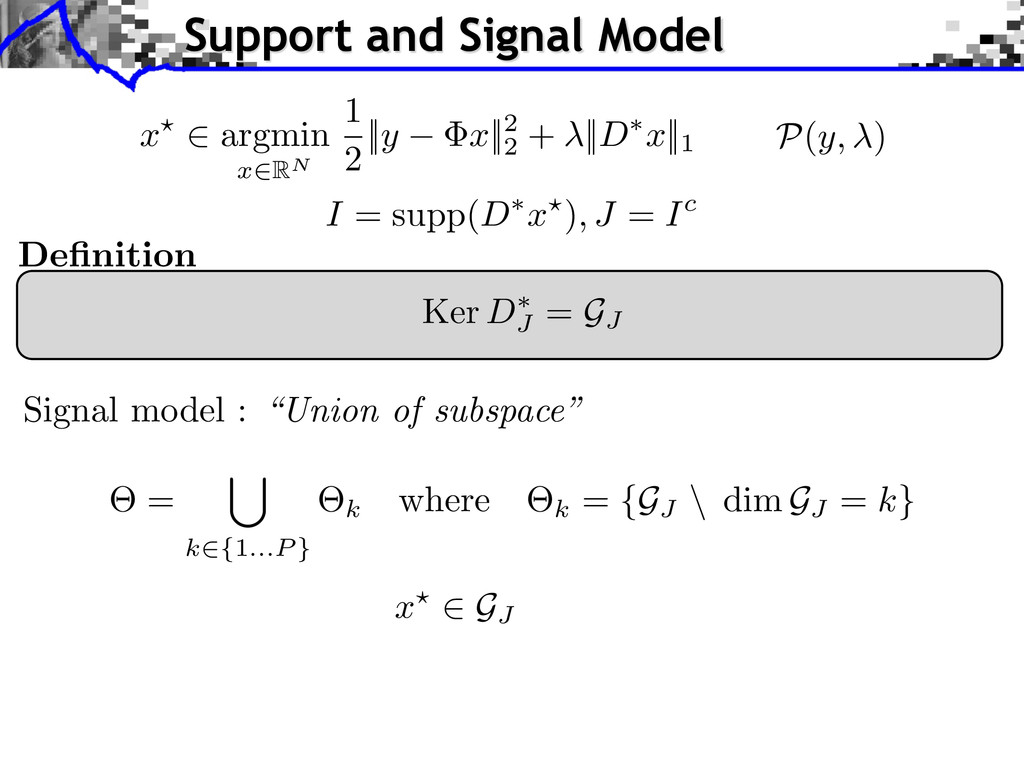
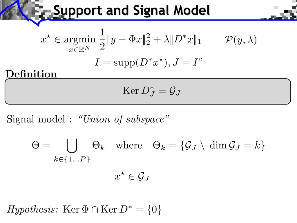
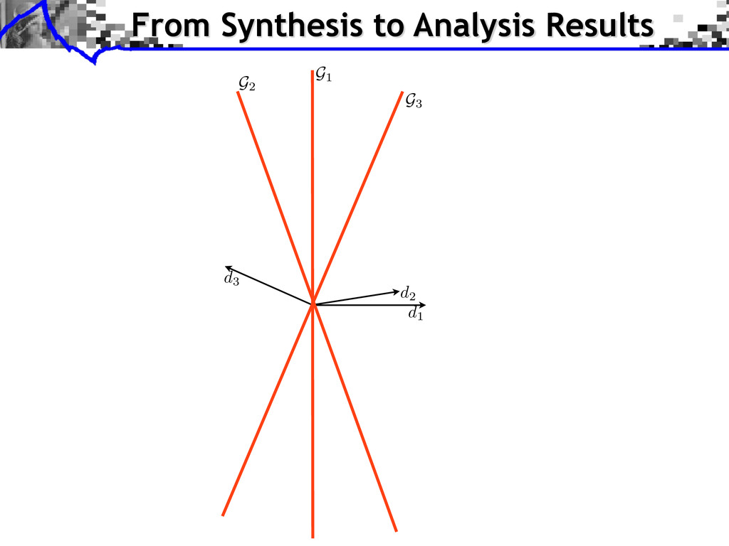
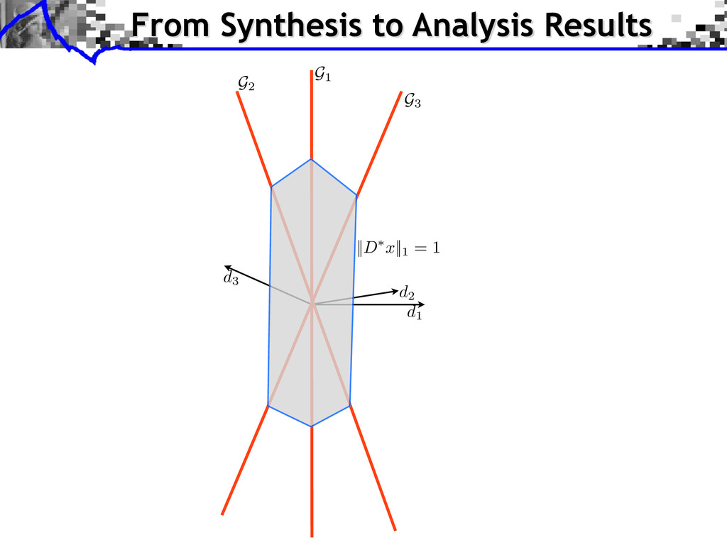
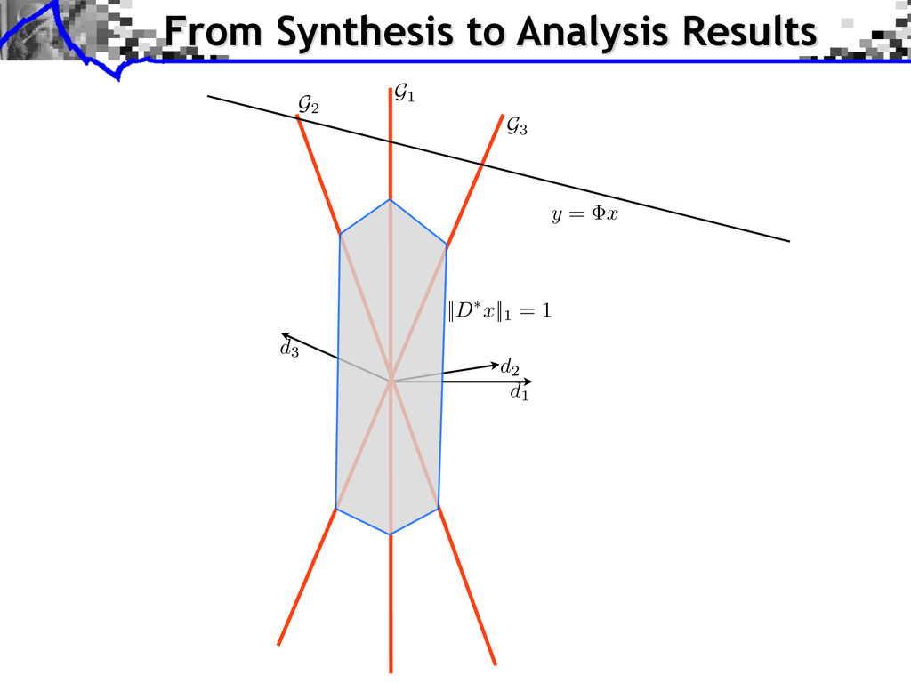
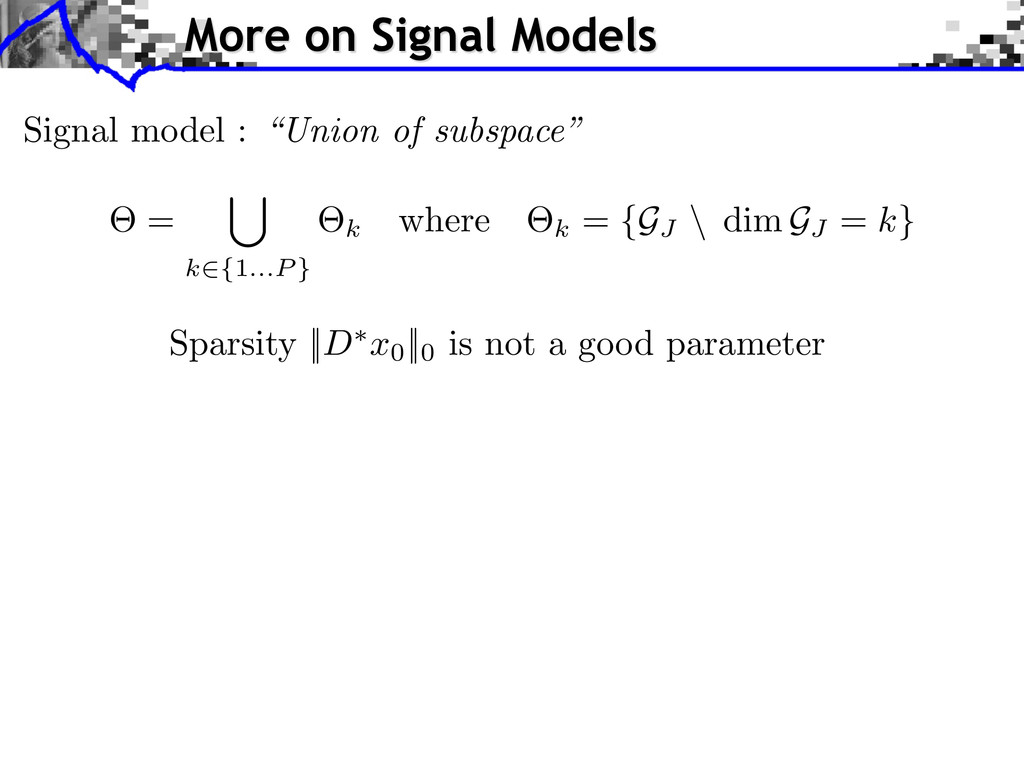
I = supp( D ⇤ x ?) , J = I c x? 2 argmin x 2RN 1 2 || y x ||2 2 + || D ⇤ x ||1 P(y, ) x ? 2 GJ ⇥ = [ k2{1...P } ⇥k where ⇥k = {GJ \ dim GJ = k} Signal model : “Union of subspace”
D⇤ = {0} Support and Signal Model I = supp( D ⇤ x ?) , J = I c x? 2 argmin x 2RN 1 2 || y x ||2 2 + || D ⇤ x ||1 P(y, ) x ? 2 GJ ⇥ = [ k2{1...P } ⇥k where ⇥k = {GJ \ dim GJ = k} Signal model : “Union of subspace”
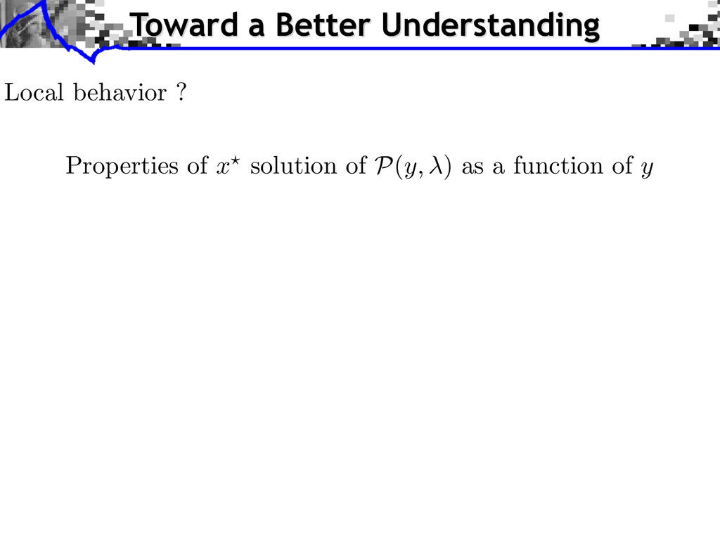
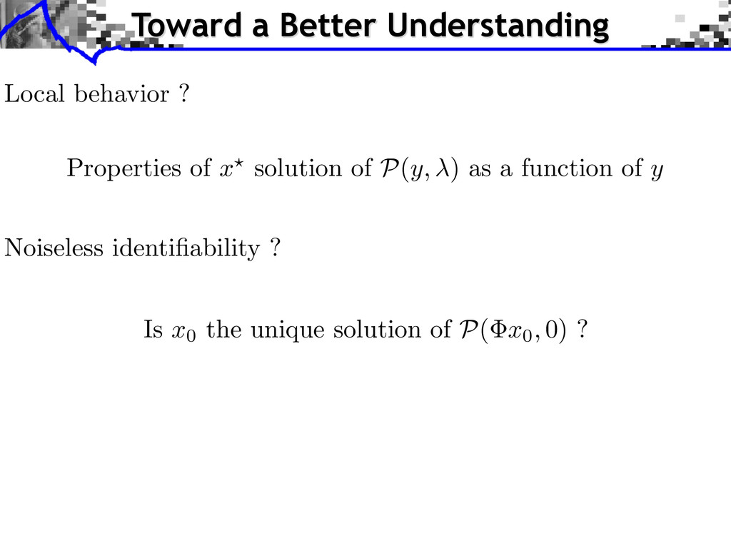
? x0 || for noisy observations ? Local behavior ? Properties of x ? solution of P (y, ) as a function of y Noiseless identifiability ? Is x0 the unique solution of P ( x0, 0) ? Toward a Better Understanding
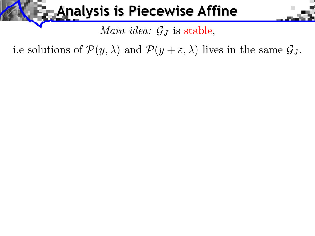
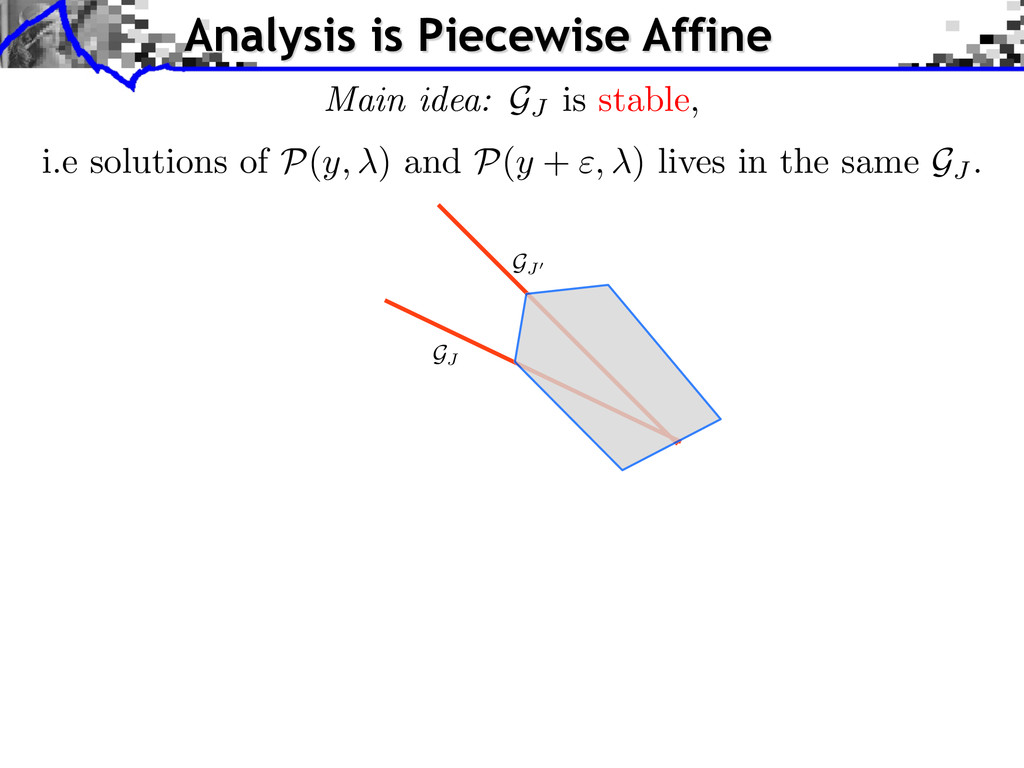
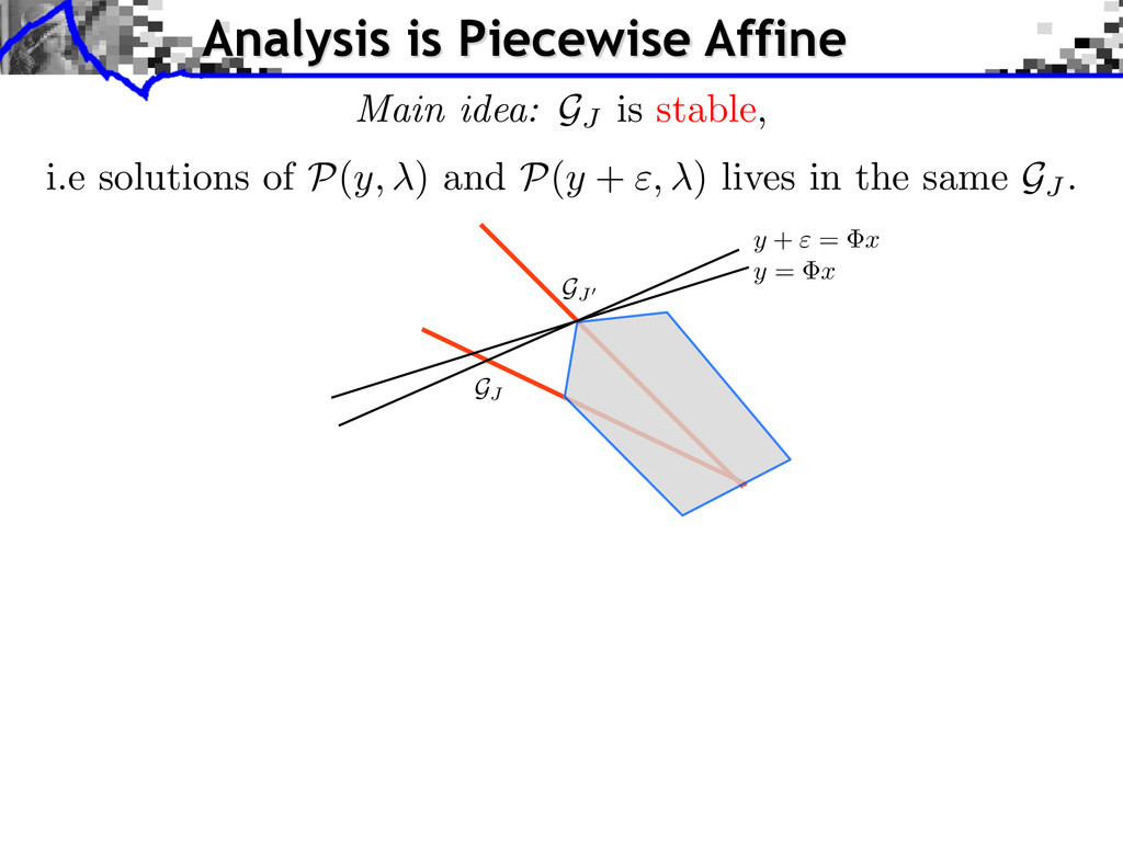
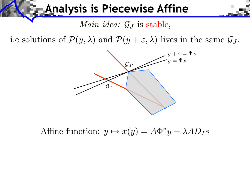
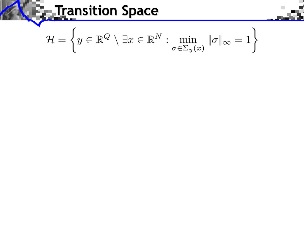
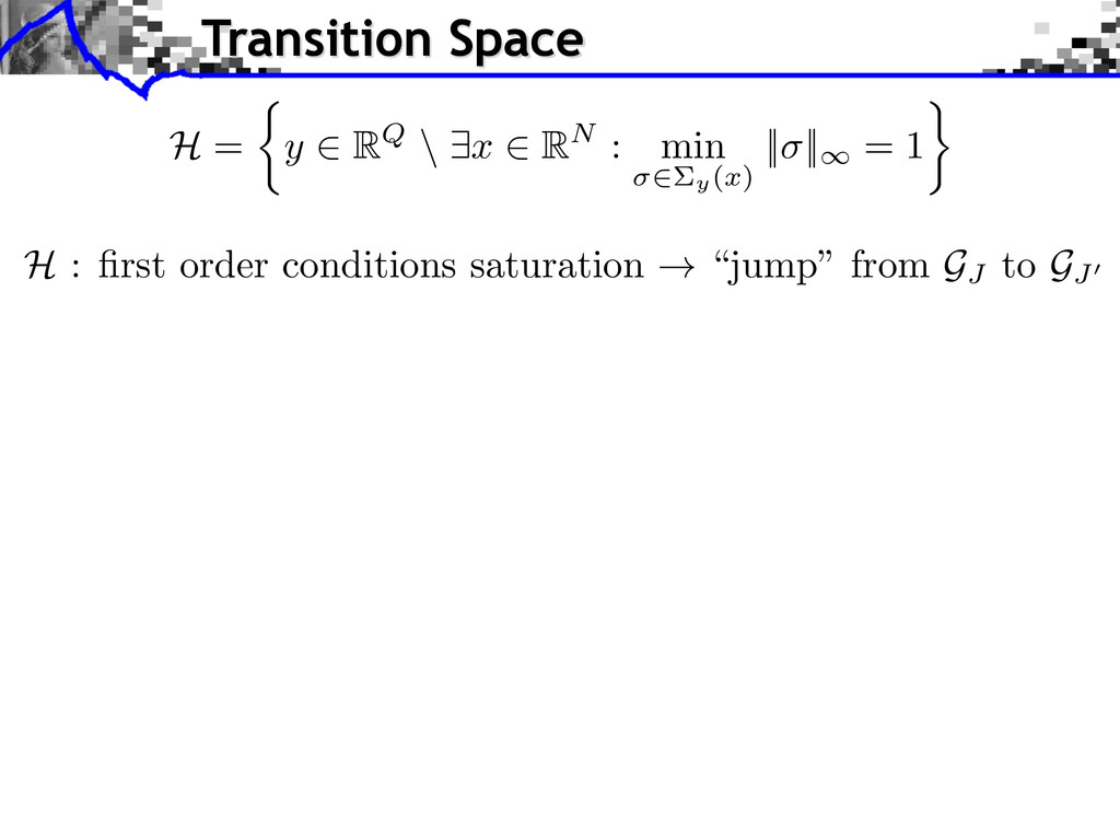
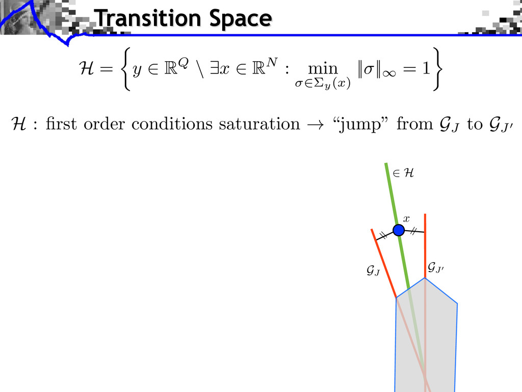
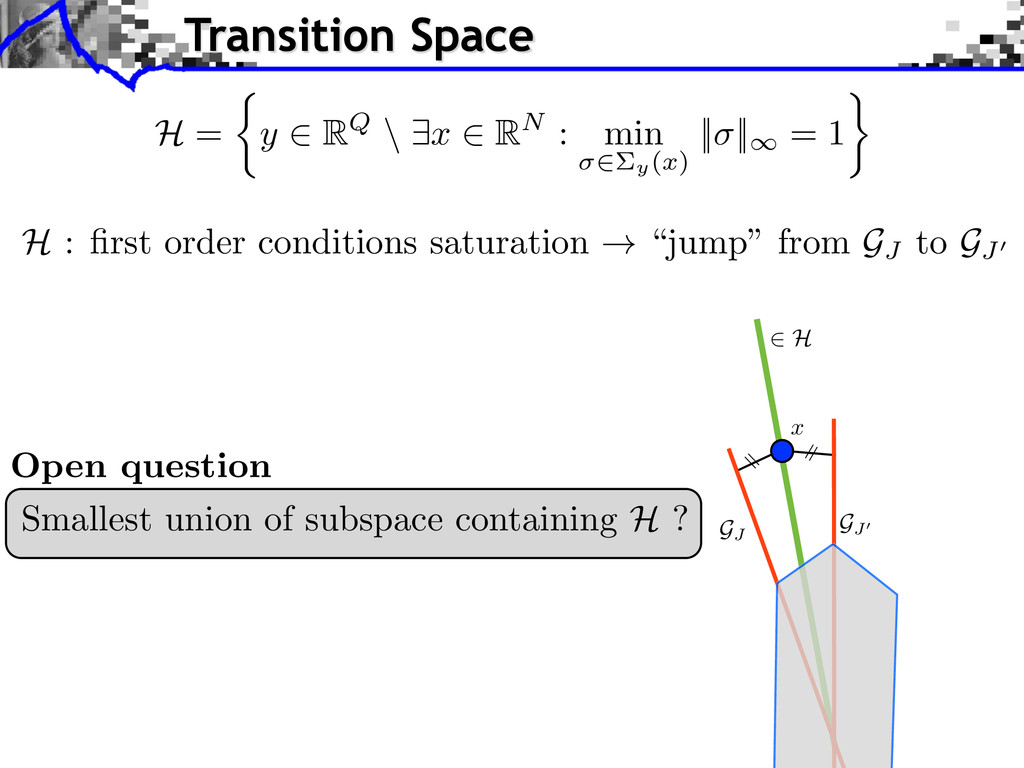
⇤ ¯ y ADI s Analysis is Piecewise Affine i.e solutions of P ( y, ) and P ( y + ", ) lives in the same GJ . Main idea: GJ is stable, GJ GJ0 y + " = x y = x
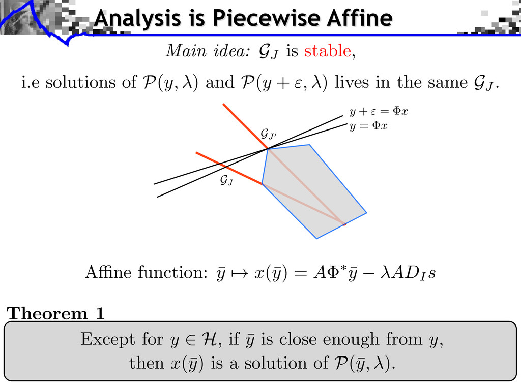
close enough from y , then x(¯ y) is a solution of P (¯ y, ). Theorem 1 A ne function: ¯ y 7! x(¯ y) = A ⇤ ¯ y ADI s Analysis is Piecewise Affine i.e solutions of P ( y, ) and P ( y + ", ) lives in the same GJ . Main idea: GJ is stable, GJ GJ0 y + " = x y = x
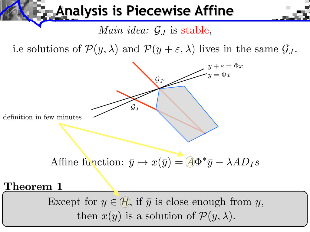
close enough from y , then x(¯ y) is a solution of P (¯ y, ). Theorem 1 A ne function: ¯ y 7! x(¯ y) = A ⇤ ¯ y ADI s Analysis is Piecewise Affine i.e solutions of P ( y, ) and P ( y + ", ) lives in the same GJ . Main idea: GJ is stable, definition in few minutes GJ GJ0 y + " = x y = x
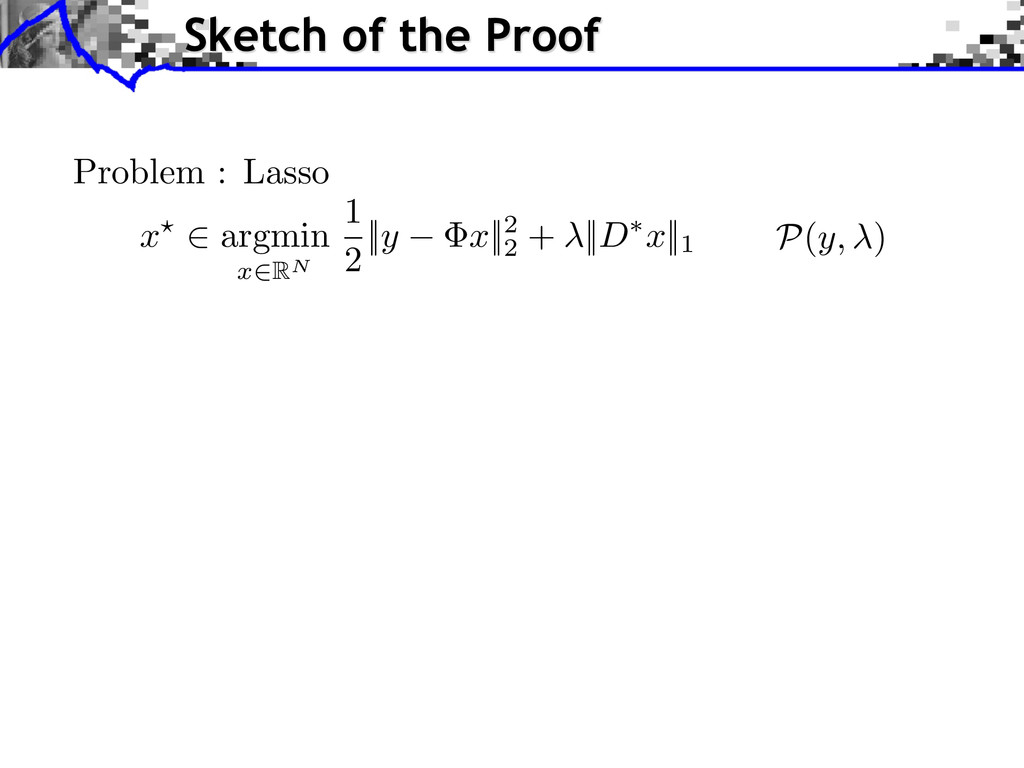
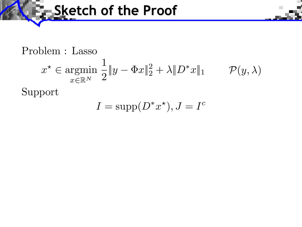
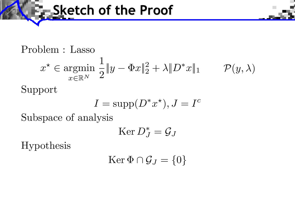
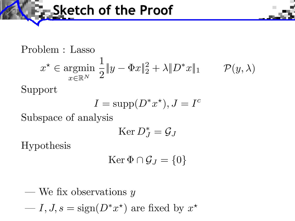
Support I = supp( D ⇤ x ?) , J = I c Problem : Lasso x? 2 argmin x 2RN 1 2 || y x ||2 2 + || D ⇤ x ||1 P(y, ) Subspace of analysis Ker D⇤ J = GJ — I, J, s = sign(D ⇤ x ? ) are fixed by x ? — We fix observations y
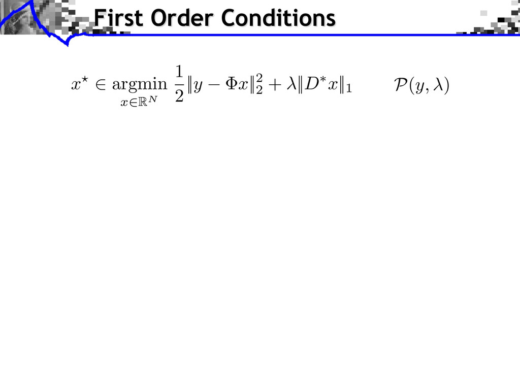
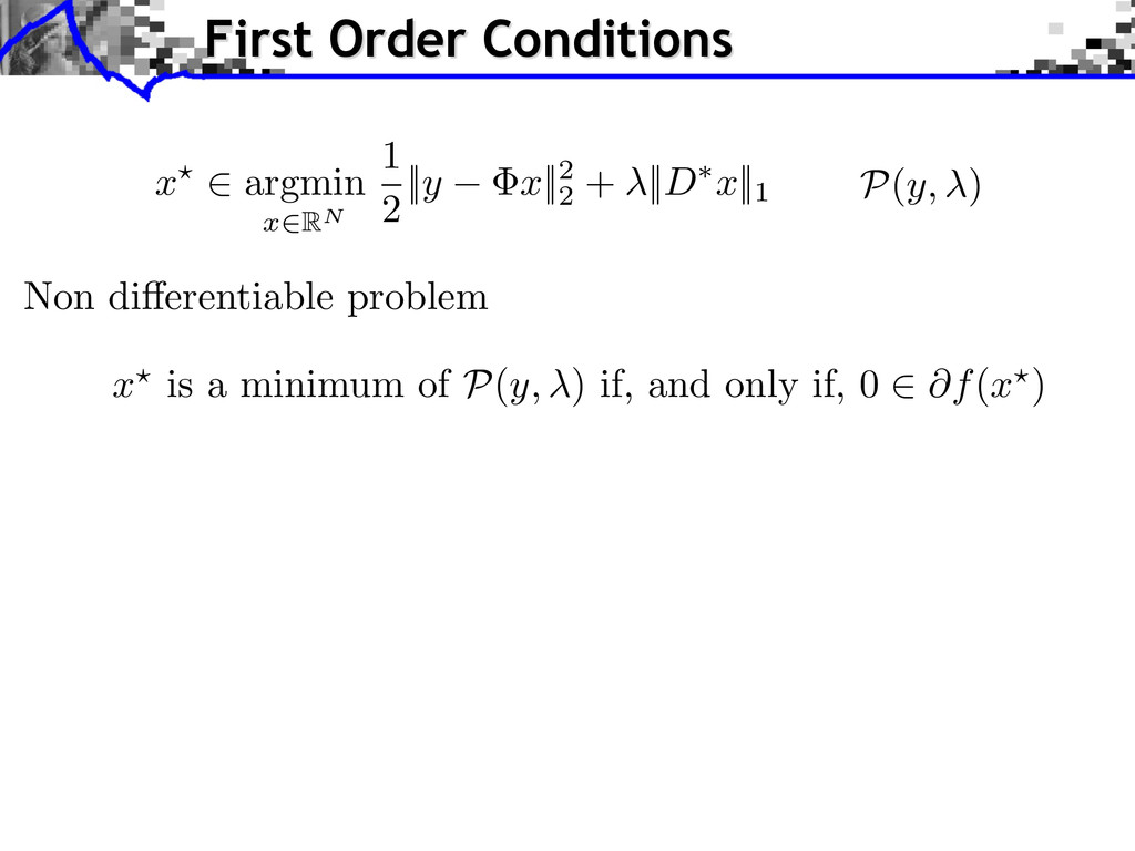
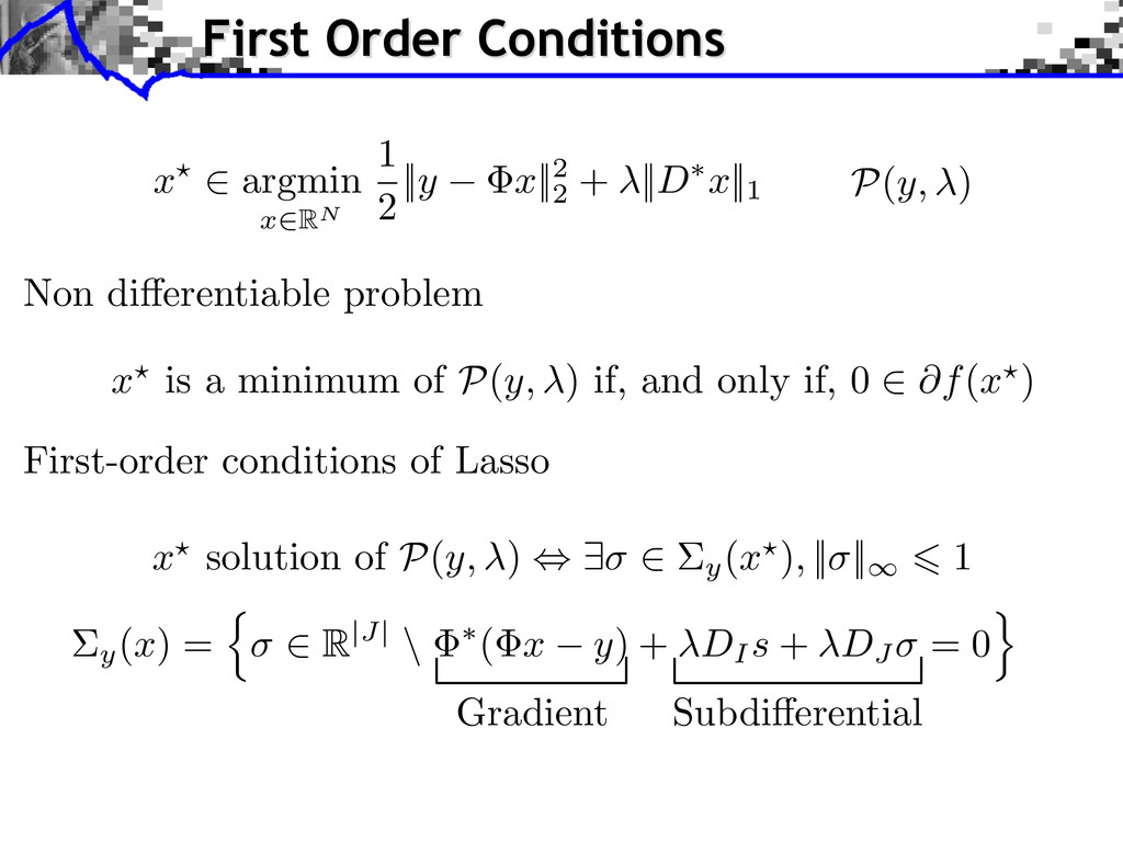
(y, ) if, and only if, 0 2 @f(x ? ) First Order Conditions x? 2 argmin x 2RN 1 2 || y x ||2 2 + || D ⇤ x ||1 P(y, ) x ? solution of P (y, ) , 9 2 ⌃y(x ? ), || ||1 6 1 ⌃y( x ) = n 2 R|J| \ ⇤( x y ) + DI s + DJ = 0o First-order conditions of Lasso Gradient Subdi↵erential
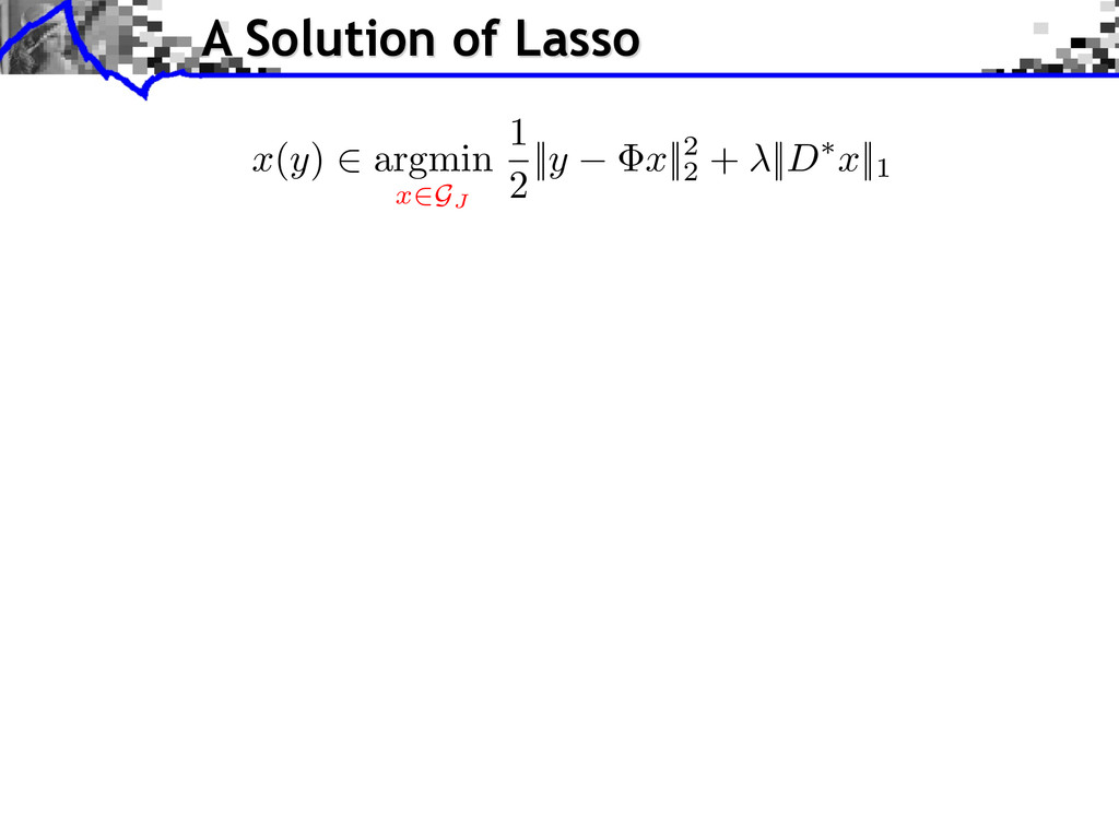
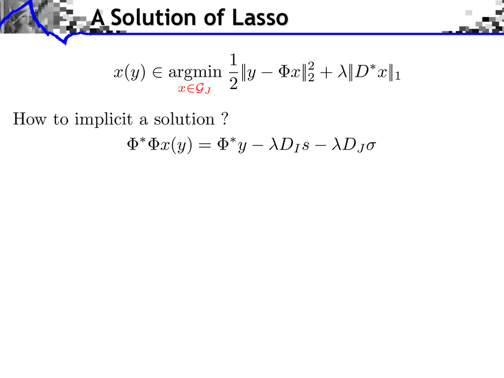
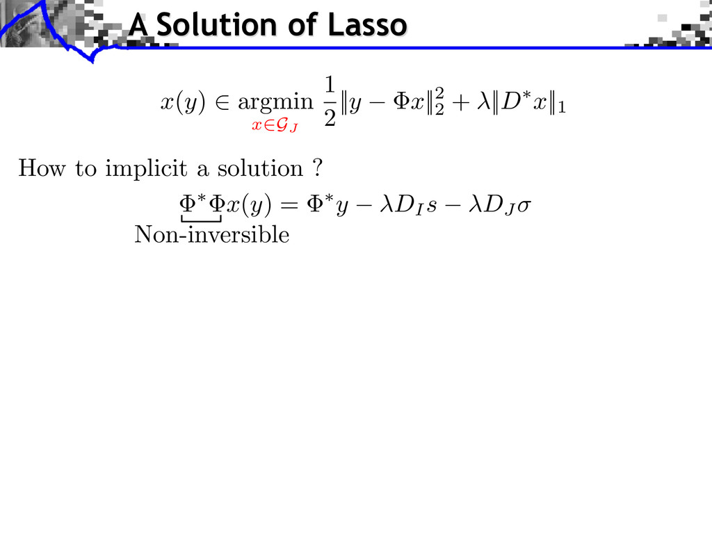
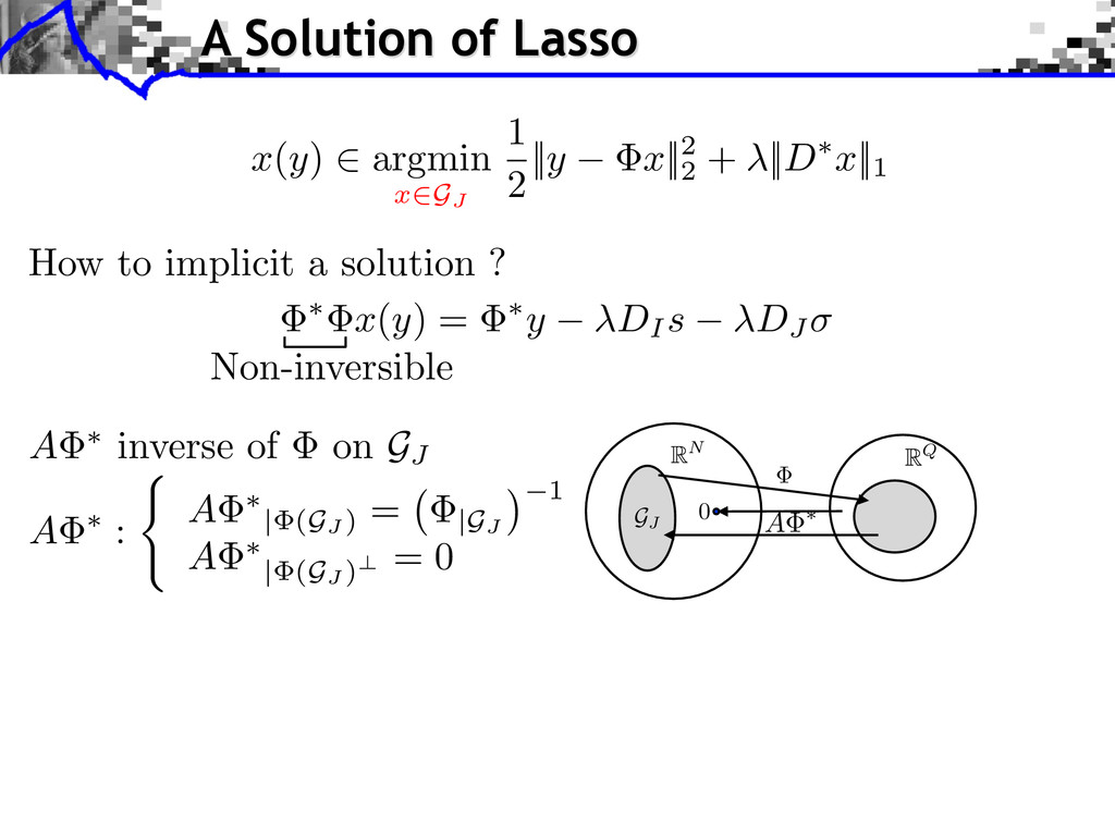
DJ x ( y ) 2 argmin x 2GJ 1 2 || y x ||2 2 + || D ⇤ x ||1 How to implicit a solution ? A Solution of Lasso A ⇤ : ( A ⇤ | (GJ ) = |GJ 1 A ⇤ | (GJ )? = 0 A ⇤ inverse of on GJ A ⇤ RQ RN 0 GJ Non-inversible
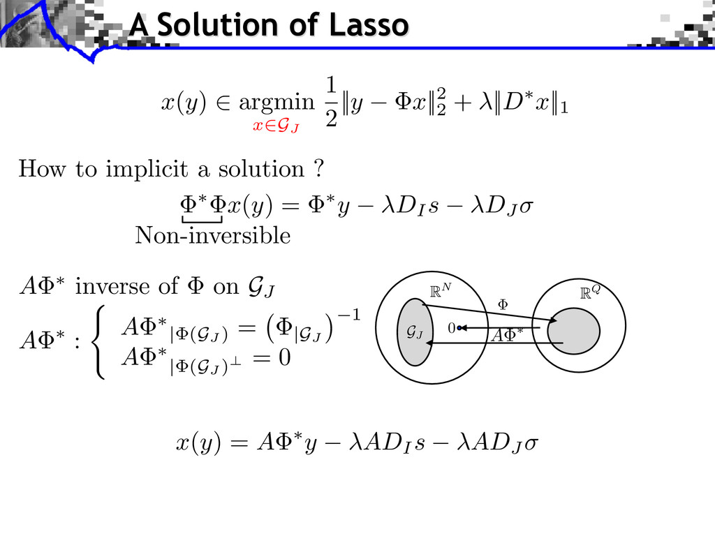
DJ x ( y ) 2 argmin x 2GJ 1 2 || y x ||2 2 + || D ⇤ x ||1 How to implicit a solution ? x ( y ) = A ⇤ y ADI s ADJ A Solution of Lasso A ⇤ : ( A ⇤ | (GJ ) = |GJ 1 A ⇤ | (GJ )? = 0 A ⇤ inverse of on GJ A ⇤ RQ RN 0 GJ Non-inversible
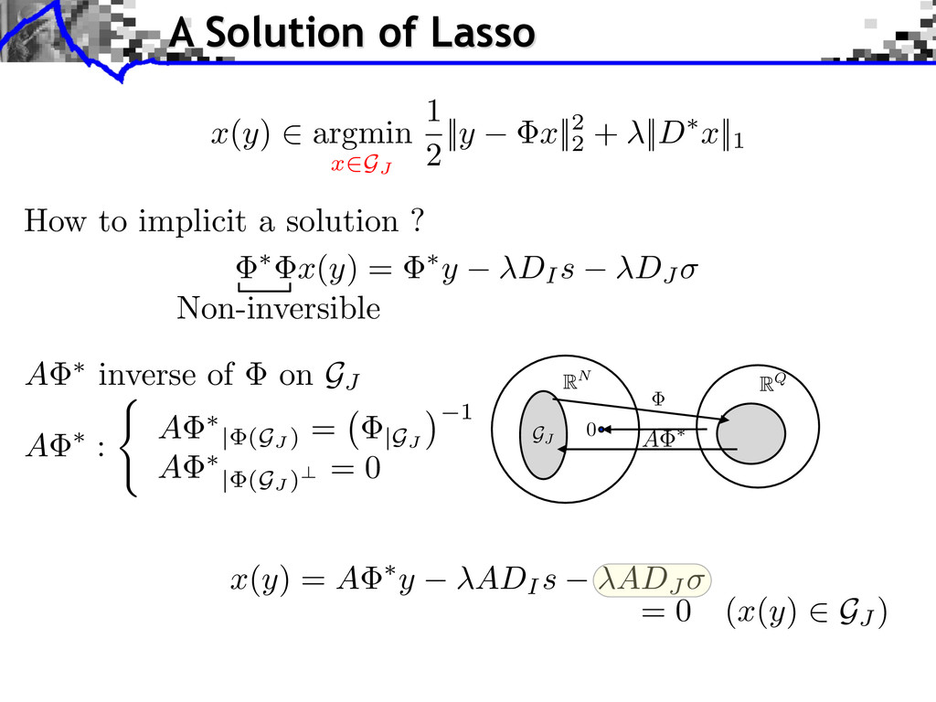
DJ x ( y ) 2 argmin x 2GJ 1 2 || y x ||2 2 + || D ⇤ x ||1 How to implicit a solution ? x ( y ) = A ⇤ y ADI s ADJ A Solution of Lasso A ⇤ : ( A ⇤ | (GJ ) = |GJ 1 A ⇤ | (GJ )? = 0 A ⇤ inverse of on GJ A ⇤ RQ RN 0 GJ Non-inversible = 0 ( x ( y ) 2 GJ )
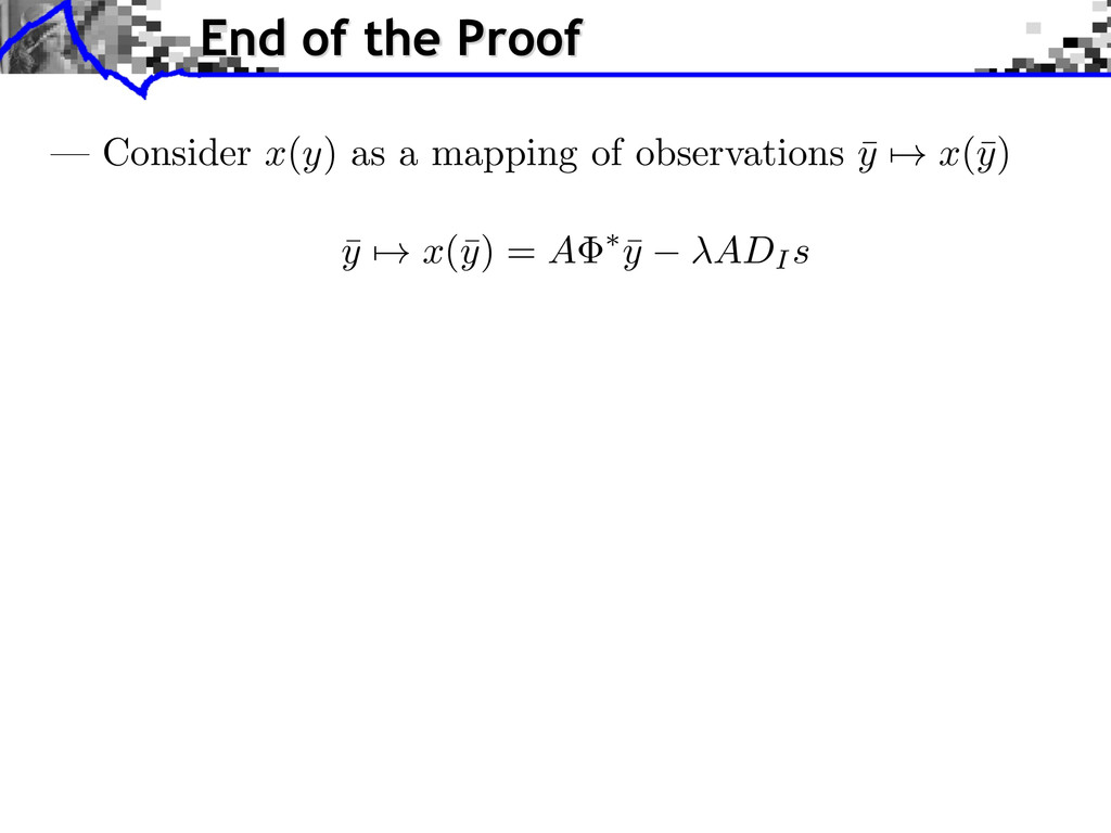
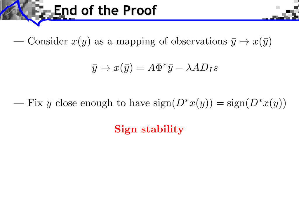
¯ y ADI s — Consider x(y) as a mapping of observations ¯ y 7! x(¯ y) — Fix ¯ y close enough to have sign(D ⇤ x(y)) = sign(D ⇤ x(¯ y)) Sign stability End of the Proof
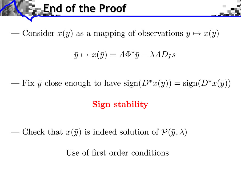
¯ y ADI s — Consider x(y) as a mapping of observations ¯ y 7! x(¯ y) — Check that x(¯ y) is indeed solution of P (¯ y, ) Use of first order conditions — Fix ¯ y close enough to have sign(D ⇤ x(y)) = sign(D ⇤ x(¯ y)) Sign stability End of the Proof
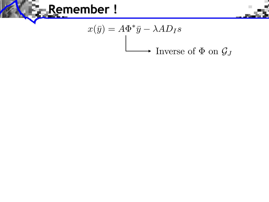
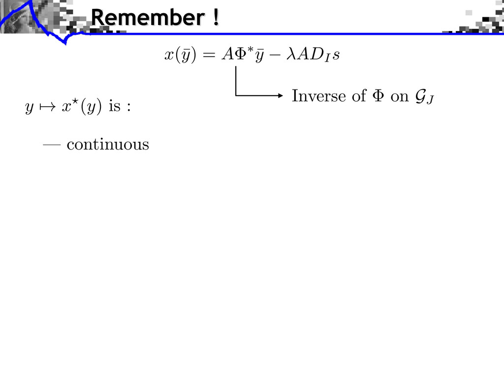
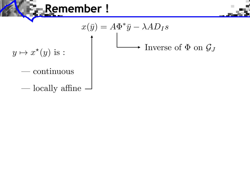
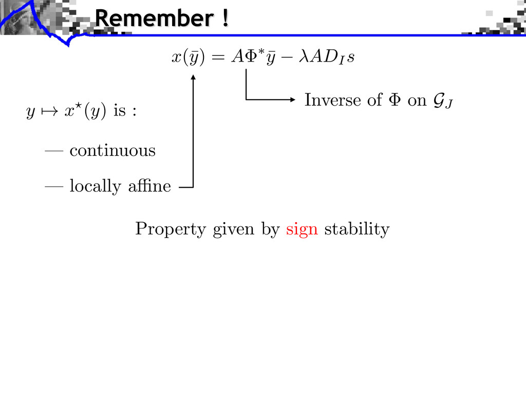
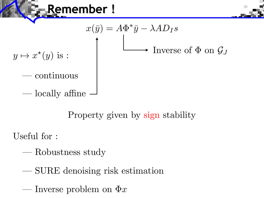
Property given by sign stability Useful for : — Robustness study — SURE denoising risk estimation — Inverse problem on x x (¯ y ) = A ⇤ ¯ y ADI s Remember ! Inverse of on GJ — locally a ne
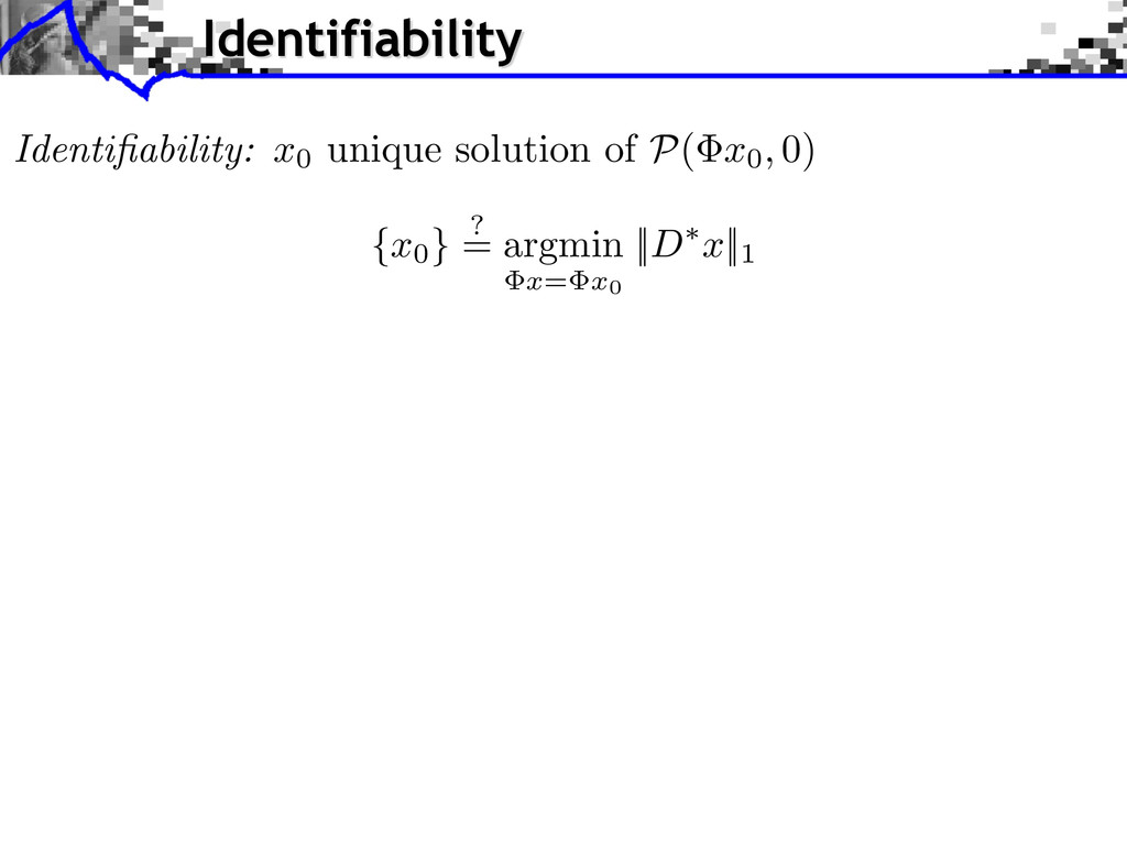
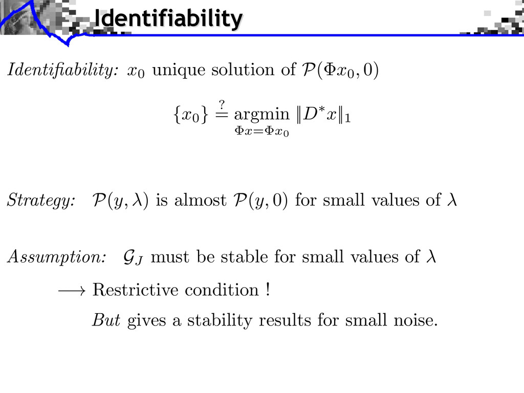
x0 } ? = argmin x = x0 || D ⇤ x ||1 ! Restrictive condition ! But gives a stability results for small noise. Assumption: GJ must be stable for small values of Strategy: P ( y, ) is almost P ( y, 0) for small values of Identifiability
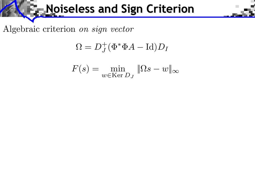
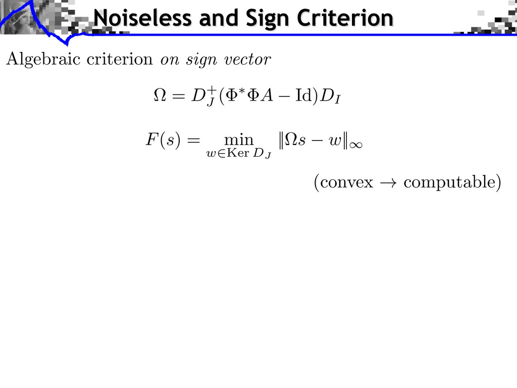
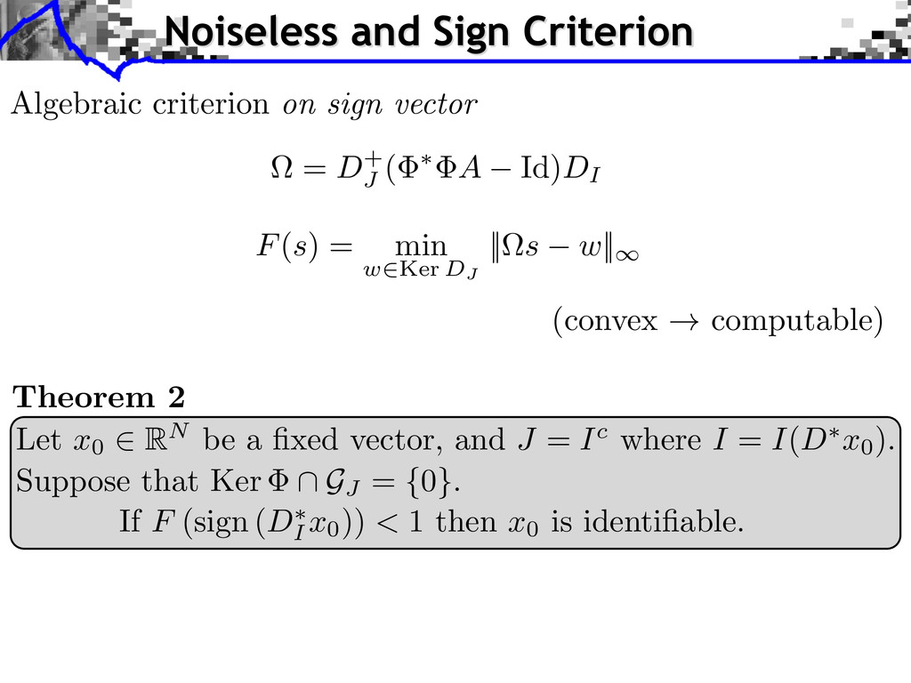
min w2Ker DJ ||⌦s w||1 Algebraic criterion on sign vector (convex ! computable) If F (sign ( D ⇤ I x0)) < 1 then x0 is identifiable. Let x0 2 RN be a fixed vector, and J = I c where I = I(D ⇤ x0). Theorem 2 Suppose that Ker \ GJ = { 0 } . Noiseless and Sign Criterion
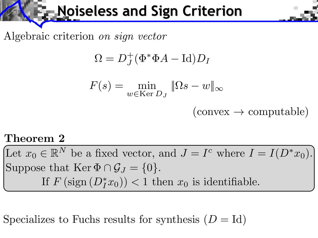
min w2Ker DJ ||⌦s w||1 Algebraic criterion on sign vector (convex ! computable) If F (sign ( D ⇤ I x0)) < 1 then x0 is identifiable. Let x0 2 RN be a fixed vector, and J = I c where I = I(D ⇤ x0). Theorem 2 Suppose that Ker \ GJ = { 0 } . Specializes to Fuchs results for synthesis ( D = Id) Noiseless and Sign Criterion
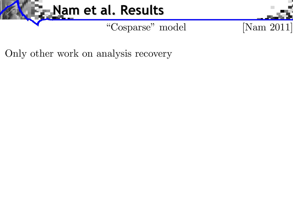
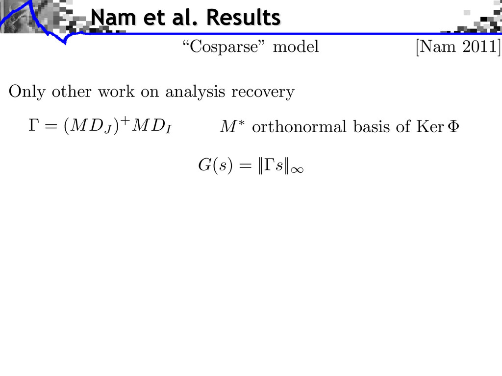
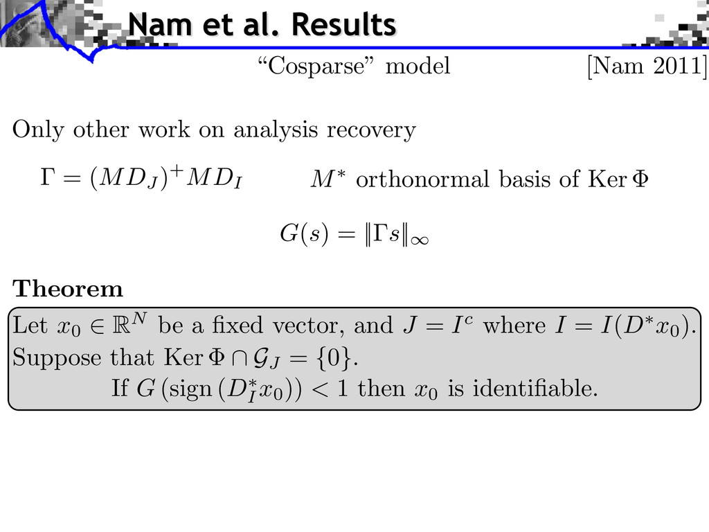
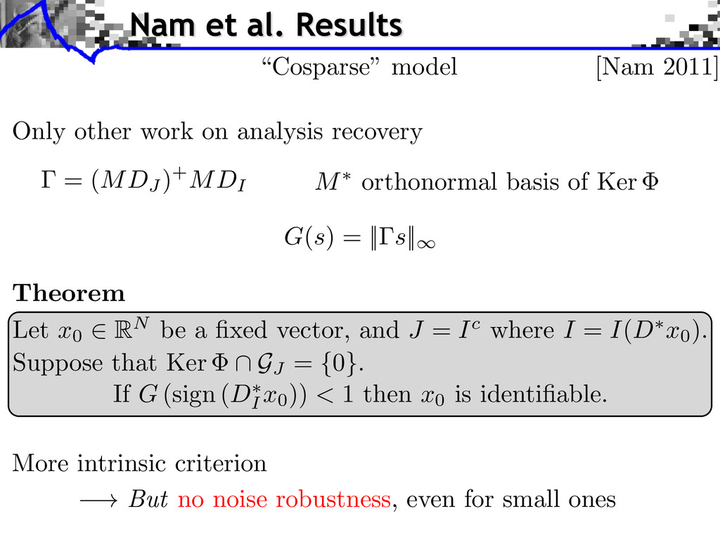
basis of Ker = (MDJ )+MDI Only other work on analysis recovery [Nam 2011] “Cosparse” model Theorem Let x0 2 RN be a fixed vector, and J = I c where I = I(D ⇤ x0). Suppose that Ker \ GJ = { 0 } . If G (sign ( D ⇤ I x0)) < 1 then x0 is identifiable.
intrinsic criterion Nam et al. Results G(s) = || s||1 M⇤ orthonormal basis of Ker = (MDJ )+MDI Only other work on analysis recovery [Nam 2011] “Cosparse” model Theorem Let x0 2 RN be a fixed vector, and J = I c where I = I(D ⇤ x0). Suppose that Ker \ GJ = { 0 } . If G (sign ( D ⇤ I x0)) < 1 then x0 is identifiable.
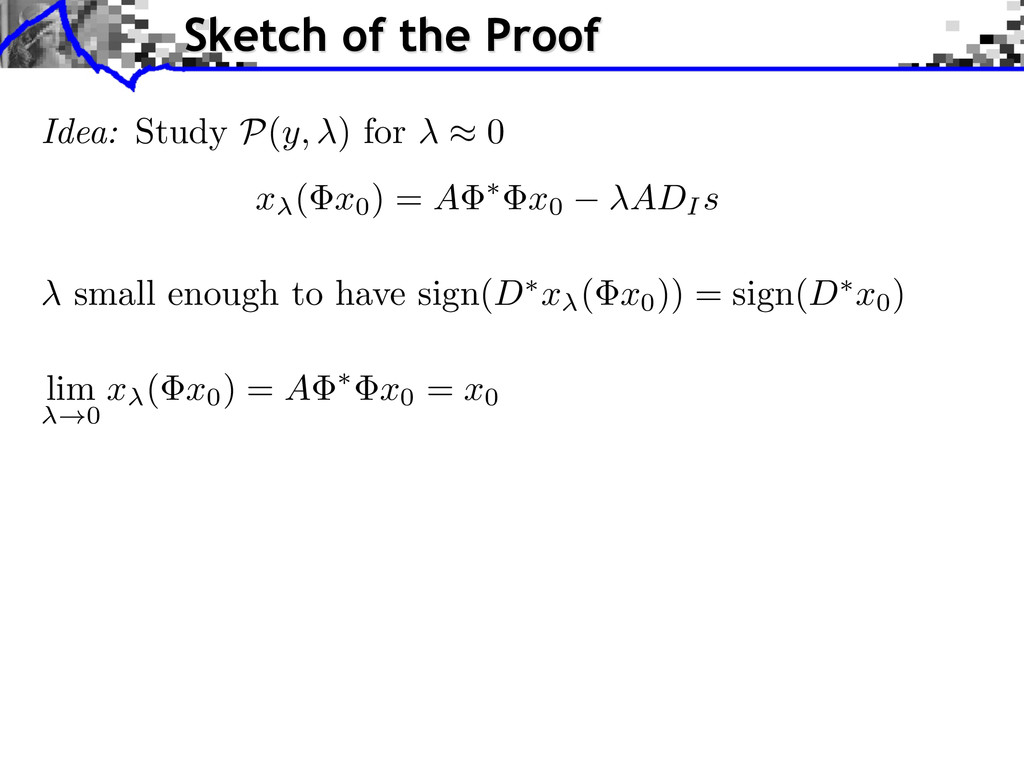
sign(D ⇤ x0) x ( x0) solution of P ( ) and x ( x0) ! !0 x0( x0) x0( x0) solution of P (0) ) x ( x0) = A ⇤ x0 ADI s Idea: Study P ( y, ) for ⇡ 0 lim !0 x ( x0) = A ⇤ x0 = x0 Sketch of the Proof
sign(D ⇤ x0) x ( x0) solution of P ( ) and x ( x0) ! !0 x0( x0) x0( x0) solution of P (0) ) x ( x0) = A ⇤ x0 ADI s Idea: Study P ( y, ) for ⇡ 0 lim !0 x ( x0) = A ⇤ x0 = x0 F(sign(D ⇤ x ( x0)) < 1 ) x ( x0) unique solution Sketch of the Proof
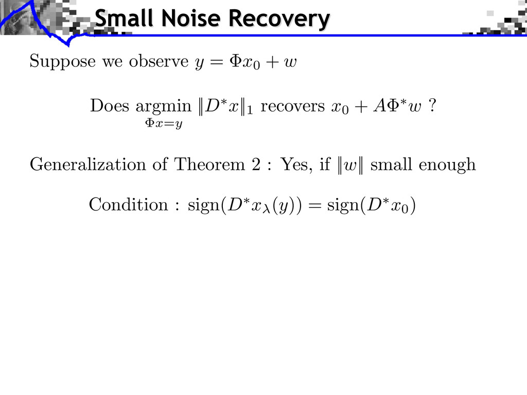
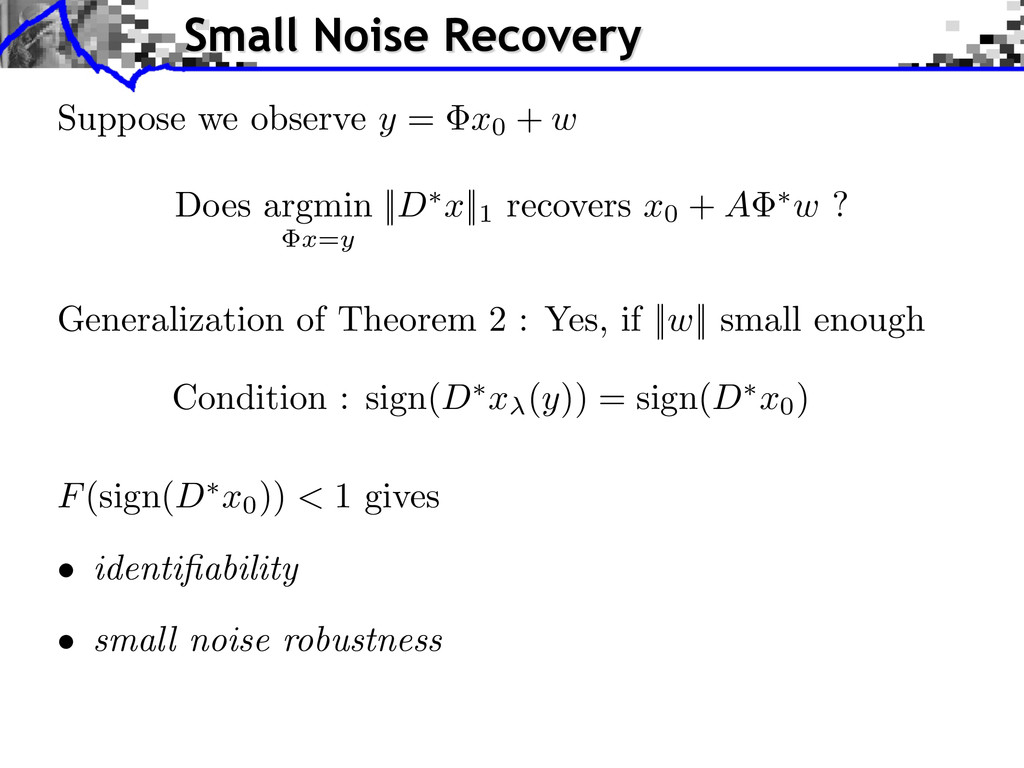
Condition : sign(D ⇤ x (y)) = sign(D ⇤ x0) F (sign( D ⇤ x0)) < 1 gives • identifiability • small noise robustness Suppose we observe y = x0 + w Does argmin x = y || D ⇤ x ||1 recovers x0 + A ⇤ w ? Small Noise Recovery
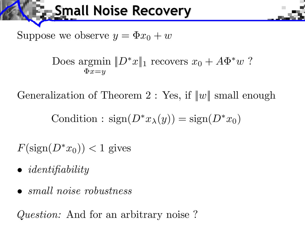
Condition : sign(D ⇤ x (y)) = sign(D ⇤ x0) Question: And for an arbitrary noise ? F (sign( D ⇤ x0)) < 1 gives • identifiability • small noise robustness Suppose we observe y = x0 + w Does argmin x = y || D ⇤ x ||1 recovers x0 + A ⇤ w ? Small Noise Recovery
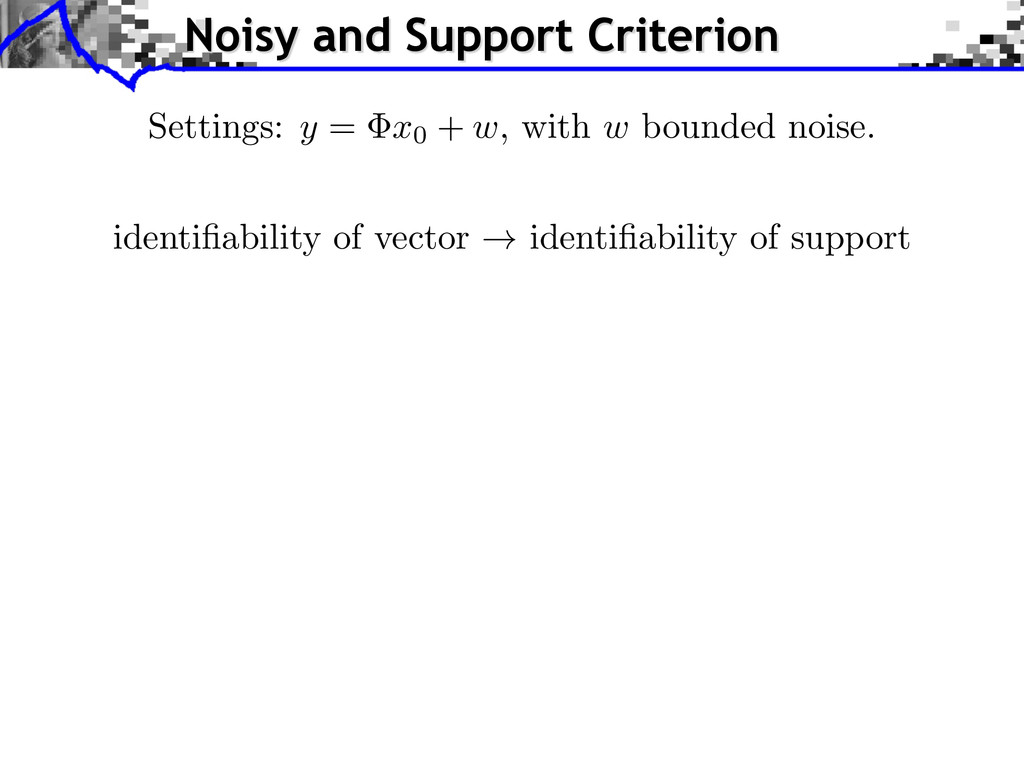
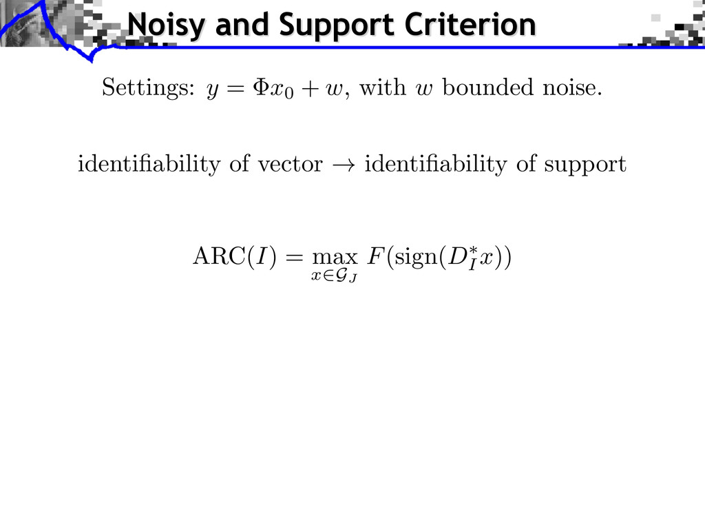
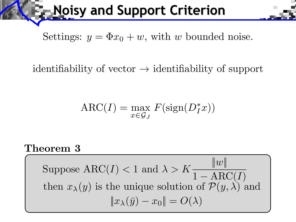
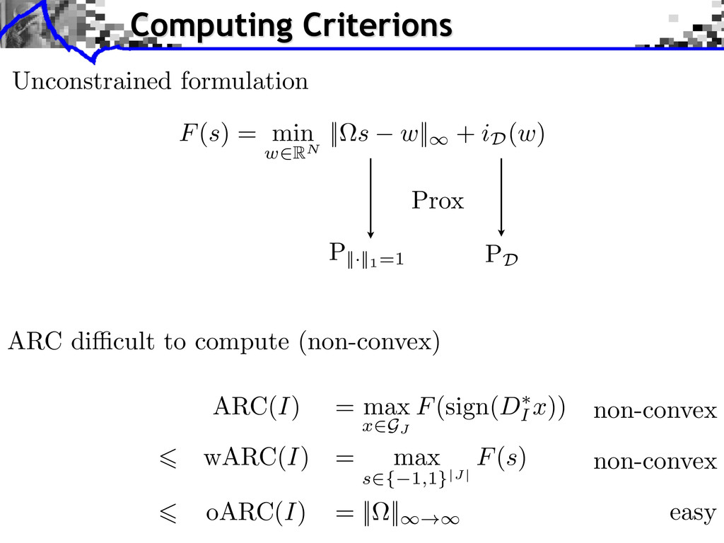
of vector ! identifiability of support Settings: y = x0 + w, with w bounded noise. then x (y) is the unique solution of P (y, ) and ||x (¯ y) x0 || = O( ) Theorem 3 Suppose ARC( I ) < 1 and > K ||w|| 1 ARC( I ) Noisy and Support Criterion
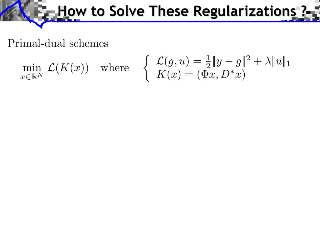
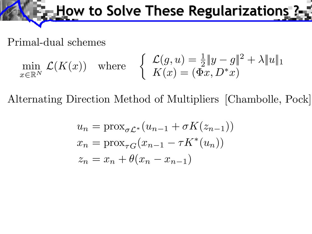
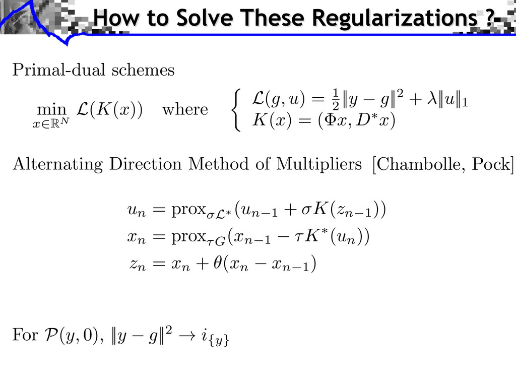
1 + K(zn 1)) xn = prox⌧G(xn 1 ⌧K ⇤ (un)) zn = xn + ✓(xn xn 1) [Chambolle, Pock] min x 2RN L( K ( x )) where ⇢ L( g, u ) = 1 2 || y g ||2 + || u ||1 K ( x ) = ( x, D ⇤ x ) Primal-dual schemes How to Solve These Regularizations ?
Direction Method of Multipliers un = prox L⇤ (un 1 + K(zn 1)) xn = prox⌧G(xn 1 ⌧K ⇤ (un)) zn = xn + ✓(xn xn 1) [Chambolle, Pock] min x 2RN L( K ( x )) where ⇢ L( g, u ) = 1 2 || y g ||2 + || u ||1 K ( x ) = ( x, D ⇤ x ) Primal-dual schemes How to Solve These Regularizations ?
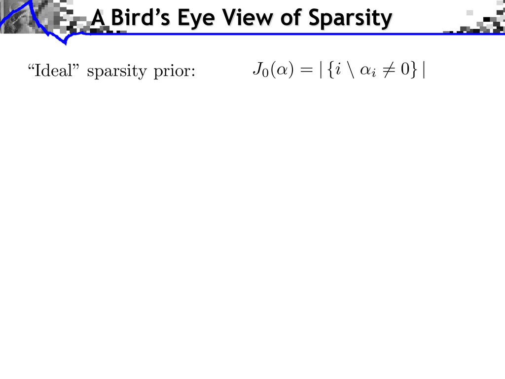
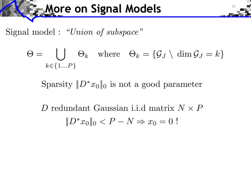
⇤ x0 ||0 < P N ) x0 = 0 ! Sparsity || D ⇤ x0 ||0 is not a good parameter More on Signal Models ⇥ = [ k2{1...P } ⇥k where ⇥k = {GJ \ dim GJ = k} Signal model : “Union of subspace”
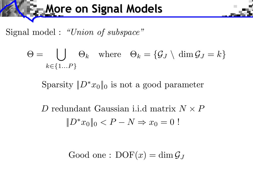
⇤ x0 ||0 < P N ) x0 = 0 ! Sparsity || D ⇤ x0 ||0 is not a good parameter Good one : DOF( x ) = dim GJ More on Signal Models ⇥ = [ k2{1...P } ⇥k where ⇥k = {GJ \ dim GJ = k} Signal model : “Union of subspace”
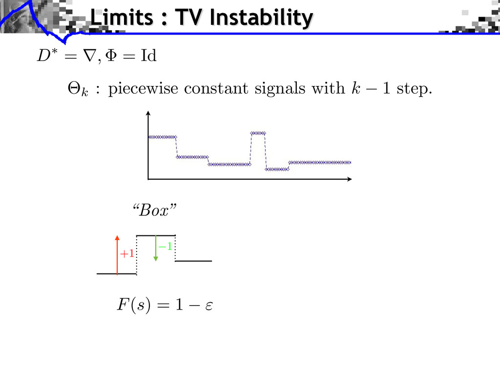
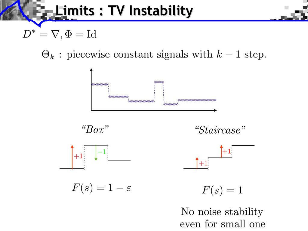
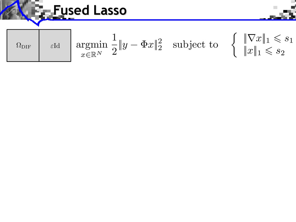
; ) 2 situations F (sign( D ⇤ x0)) > 1 no noise robustness |c b| 6 ⇠(") Fused Lasso argmin x 2RN 1 2 || y x ||2 2 subject to ⇢ ||r x ||1 6 s1 || x ||1 6 s2 "Id ⌦DIF
; ) 2 situations F (sign( D ⇤ x0)) > 1 no noise robustness |c b| 6 ⇠(") strong noise robustness F (sign( D ⇤ x0)) = ARC( I ) < 1 |c b| > ⇠(") Haar : similar results Fused Lasso argmin x 2RN 1 2 || y x ||2 2 subject to ⇢ ||r x ||1 6 s1 || x ||1 6 s2 "Id ⌦DIF
ensure noisy recovery ? What’s Next ? Deterministic theorem ! treat the noise as a random variable — Support identifiability with Gaussian, Poisson noise
ensure noisy recovery ? What’s Next ? Work initiated by Chambolle in TV — Continuous model Deterministic theorem ! treat the noise as a random variable — Support identifiability with Gaussian, Poisson noise
ensure noisy recovery ? What’s Next ? Work initiated by Chambolle in TV — Continuous model — Larger class of priors J Block sparsity || · ||p,q Deterministic theorem ! treat the noise as a random variable — Support identifiability with Gaussian, Poisson noise
ensure noisy recovery ? What’s Next ? Work initiated by Chambolle in TV — Continuous model — Larger class of priors J Block sparsity || · ||p,q — Real-world recovery results Almost equal support recovery Deterministic theorem ! treat the noise as a random variable — Support identifiability with Gaussian, Poisson noise
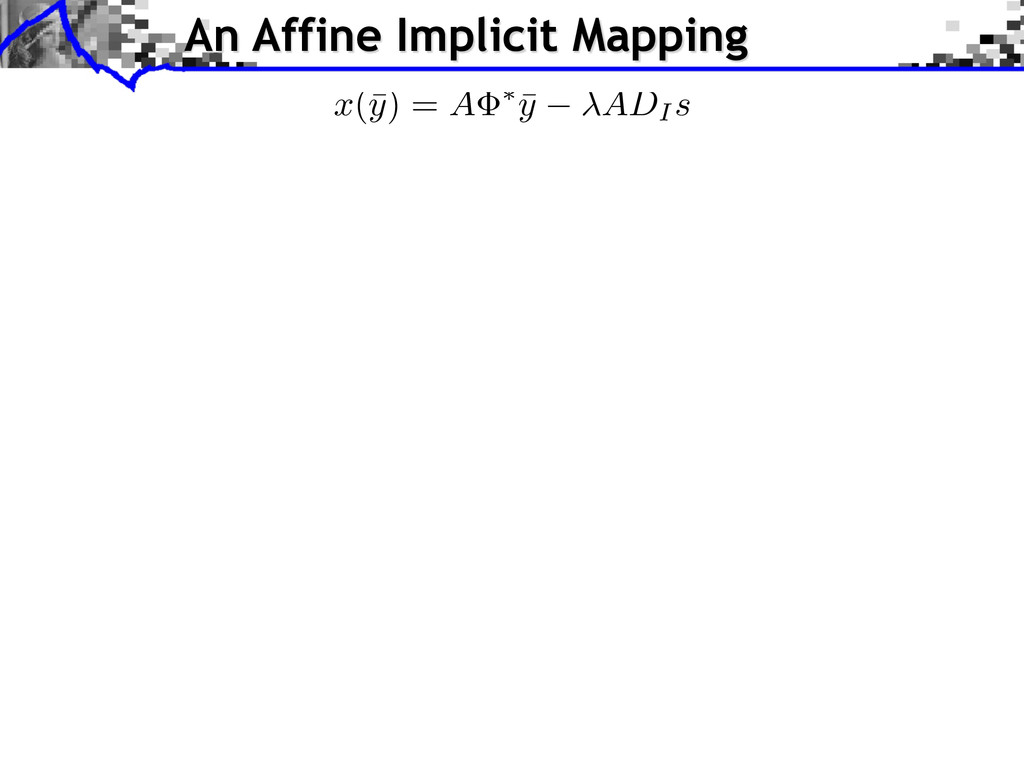
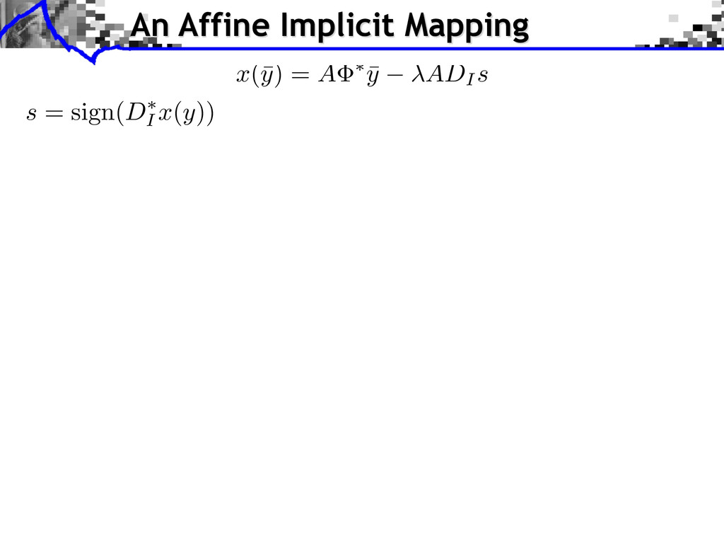
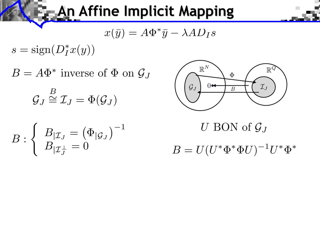
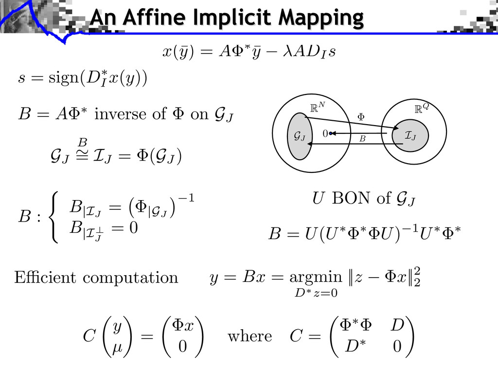
0 B = U(U⇤ ⇤ U) 1U⇤ ⇤ U BON of GJ x (¯ y ) = A ⇤ ¯ y ADI s s = sign( D ⇤ I x ( y )) An Affine Implicit Mapping B = A ⇤ inverse of on GJ GJ B ⇠ = IJ = (GJ ) B RQ RN 0 IJ GJ
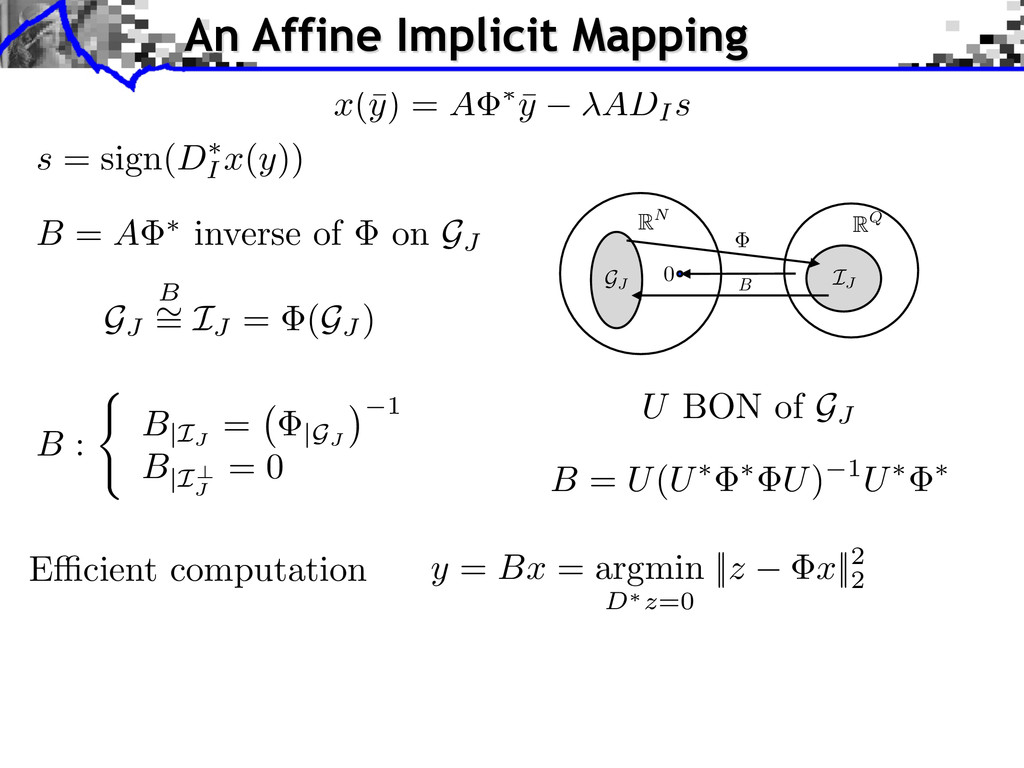
0 B = U(U⇤ ⇤ U) 1U⇤ ⇤ U BON of GJ x (¯ y ) = A ⇤ ¯ y ADI s s = sign( D ⇤ I x ( y )) E cient computation y = Bx = argmin D⇤z=0 || z x ||2 2 An Affine Implicit Mapping B = A ⇤ inverse of on GJ GJ B ⇠ = IJ = (GJ ) B RQ RN 0 IJ GJ
0 B = U(U⇤ ⇤ U) 1U⇤ ⇤ U BON of GJ x (¯ y ) = A ⇤ ¯ y ADI s s = sign( D ⇤ I x ( y )) C ✓ y µ ◆ = ✓ x 0 ◆ where C = ✓ ⇤ D D ⇤ 0 ◆ E cient computation y = Bx = argmin D⇤z=0 || z x ||2 2 An Affine Implicit Mapping B = A ⇤ inverse of on GJ GJ B ⇠ = IJ = (GJ ) B RQ RN 0 IJ GJ
![[Fuchs, Tropp, Dossal]: address these questions — Previous works in](https://files.speakerdeck.com/presentations/2bd7c73db2d54a8cae00fd3578bb3c3a/slide_41.jpg)
![[Fuchs, Tropp, Dossal]: address these questions — Previous works in](https://files.speakerdeck.com/presentations/2bd7c73db2d54a8cae00fd3578bb3c3a/slide_42.jpg)
![Signal Model: Characteristic functions sum ⇥2 : x0 = 1[a,b]](https://files.speakerdeck.com/presentations/2bd7c73db2d54a8cae00fd3578bb3c3a/slide_144.jpg)
![Signal Model: Characteristic functions sum ⇥2 : x0 = 1[a,b]](https://files.speakerdeck.com/presentations/2bd7c73db2d54a8cae00fd3578bb3c3a/slide_145.jpg)
![[ a, b ] \ [ c, d ] 6=](https://files.speakerdeck.com/presentations/2bd7c73db2d54a8cae00fd3578bb3c3a/slide_146.jpg)
![[ a, b ] \ [ c, d ] =](https://files.speakerdeck.com/presentations/2bd7c73db2d54a8cae00fd3578bb3c3a/slide_147.jpg)
![[ a, b ] \ [ c, d ] =](https://files.speakerdeck.com/presentations/2bd7c73db2d54a8cae00fd3578bb3c3a/slide_148.jpg)
![[ a, b ] \ [ c, d ] =](https://files.speakerdeck.com/presentations/2bd7c73db2d54a8cae00fd3578bb3c3a/slide_149.jpg)
![[ a, b ] \ [ c, d ] =](https://files.speakerdeck.com/presentations/2bd7c73db2d54a8cae00fd3578bb3c3a/slide_150.jpg)