#27 Transfert de style et Generative Adversarial Networks

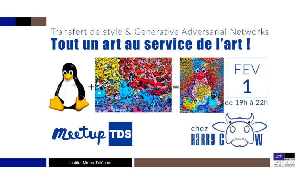
Le transfert de style est une tâche à part entière : comprendre et extraire le style d'une œuvre d'art pour l'appliquer à une photo sans modifier son contenu sémantique (objets présents dans la scène).
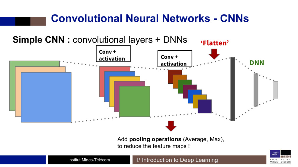
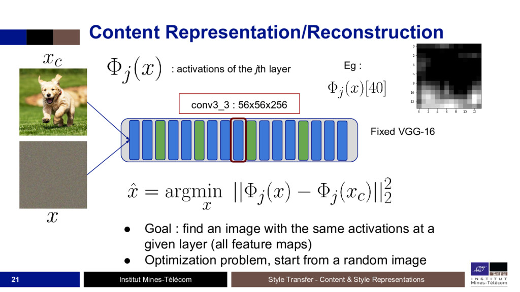
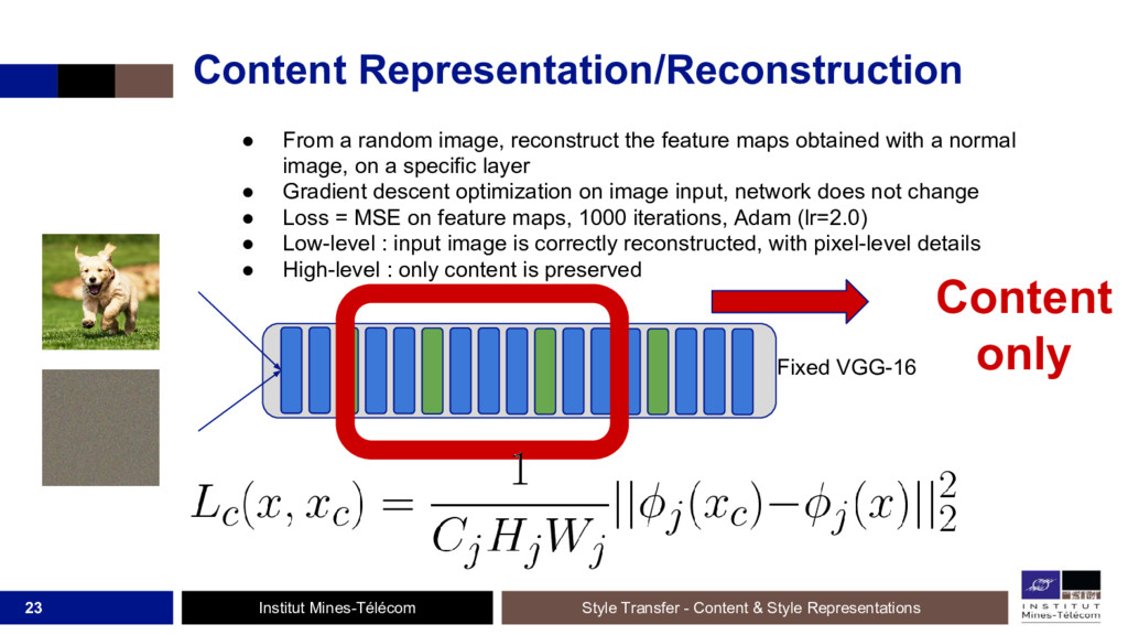
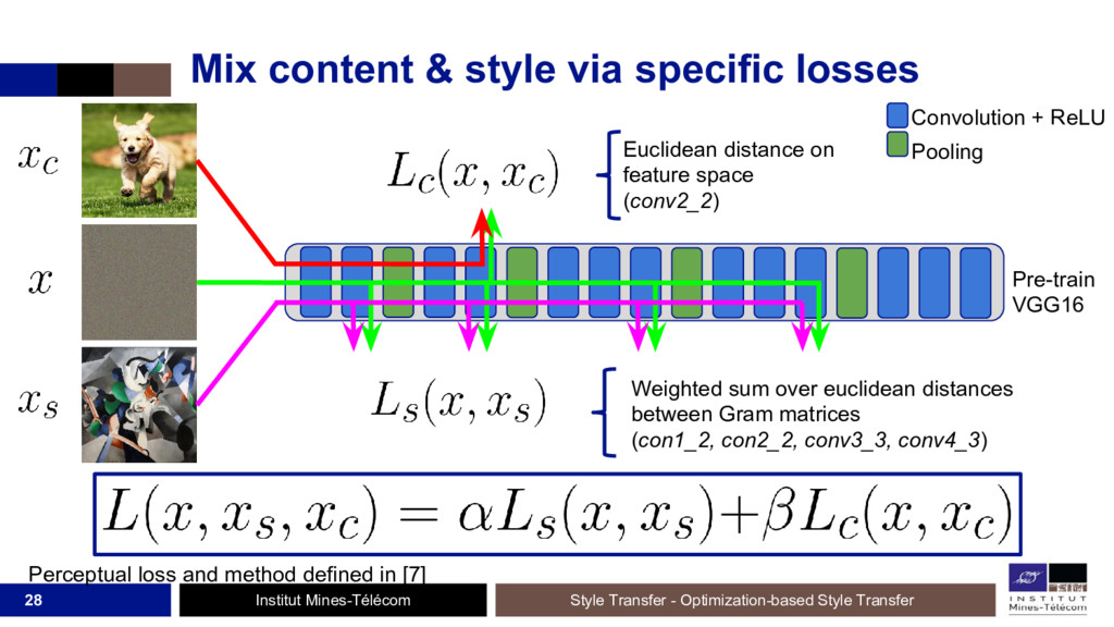
Depuis 2015, des méthodes à bases de réseaux de neurones convolutifs (CNNs) se sont mis à surpasser les précédentes techniques. Des CNNs entraînés pour la classification d'images permettent de réaliser cette opération, en définissant une fonction de coût (ou d'erreur) spécifique à la reconnaissance du style et du contenu! Un réseau de neurones sert alors de support à l'entraînement d'autres réseaux.

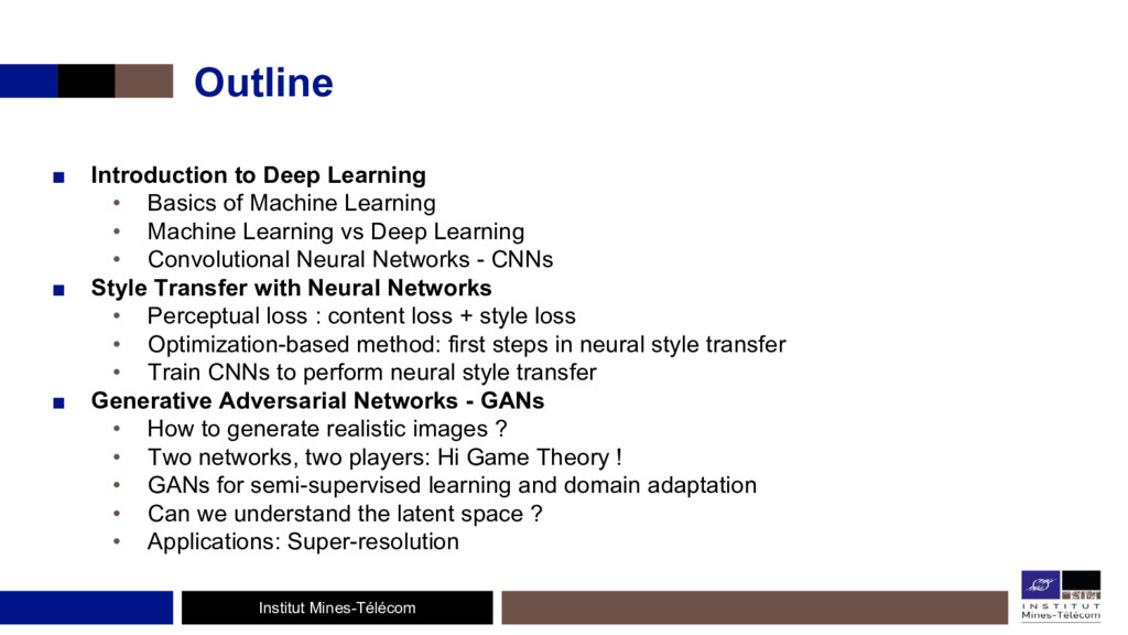
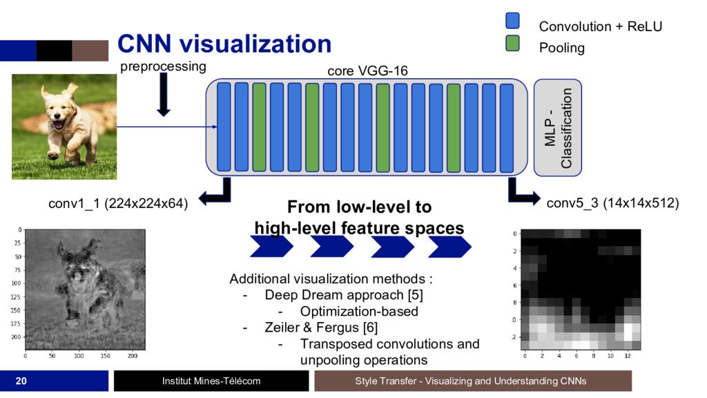
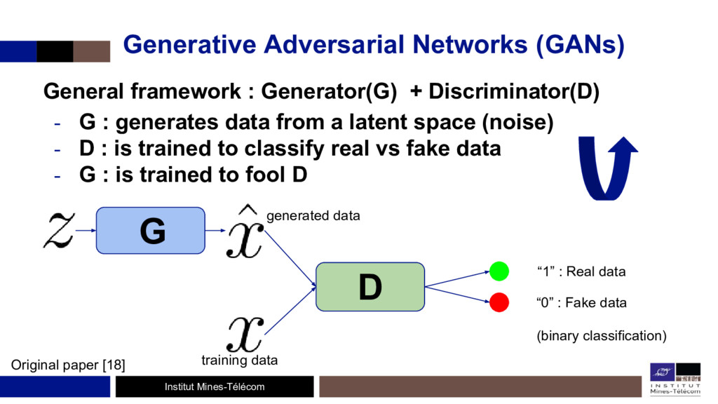
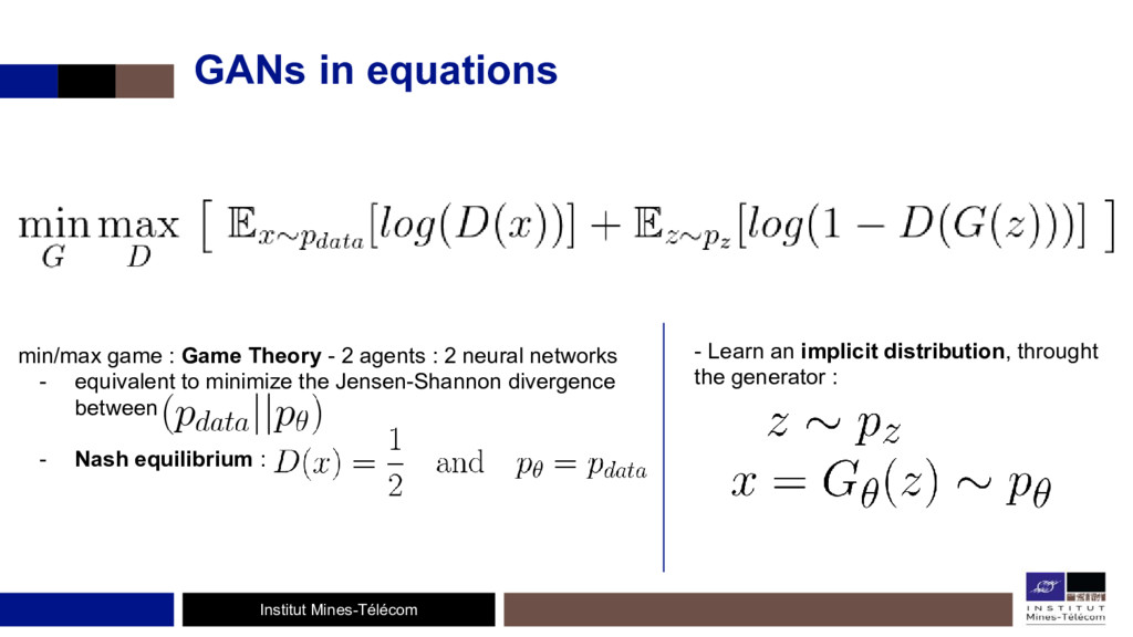
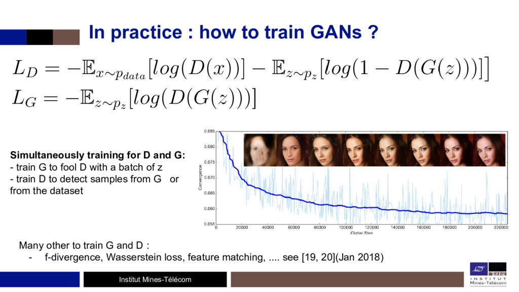
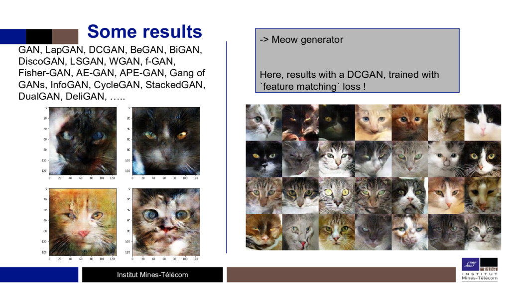
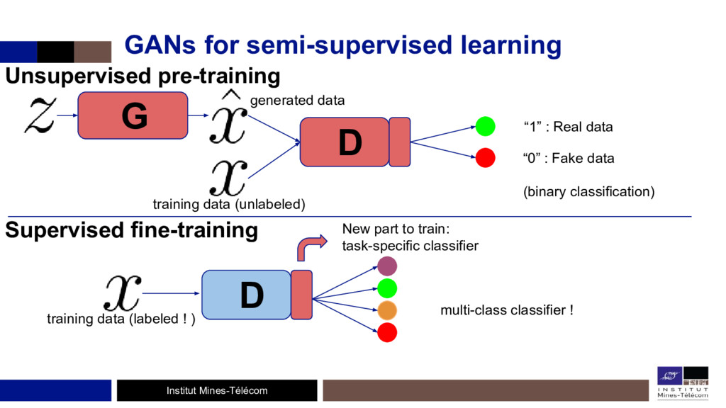
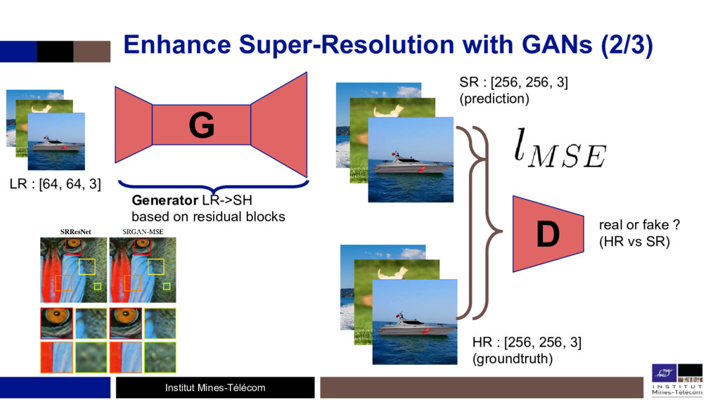
L'étude de ces algorithmes permet de bien comprendre les réseaux de neurones, de voir ce qu'il se passe à l'intérieur et de se défaire l'effet 'black-box' des CNNs. D'un autre côté, les Generative Adversarial Networks (GANs) forment un framework générique où deux réseaux de neurones, un générateur et un discriminateur, s'entraînent en même temps, de façon compétitive: le discriminateur cherchant à faire la différence entre des images réelles (provenant d'un dataset) et des images produites par le générateur, ce dernier voulant ensuite tromper le discriminateur.
Le discriminateur se comporte comme une fonction d'erreur 'entraînable' qui oblige le générateur à produire des images réalistes. Cette fonction de coût peut très bien s'ajouter à d'autres fonctions de coûts.

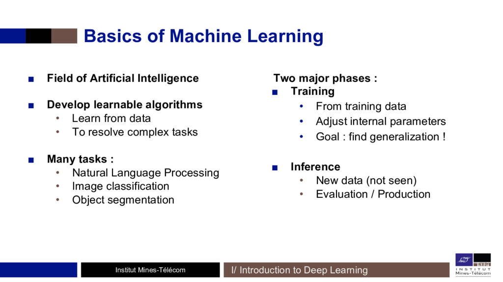
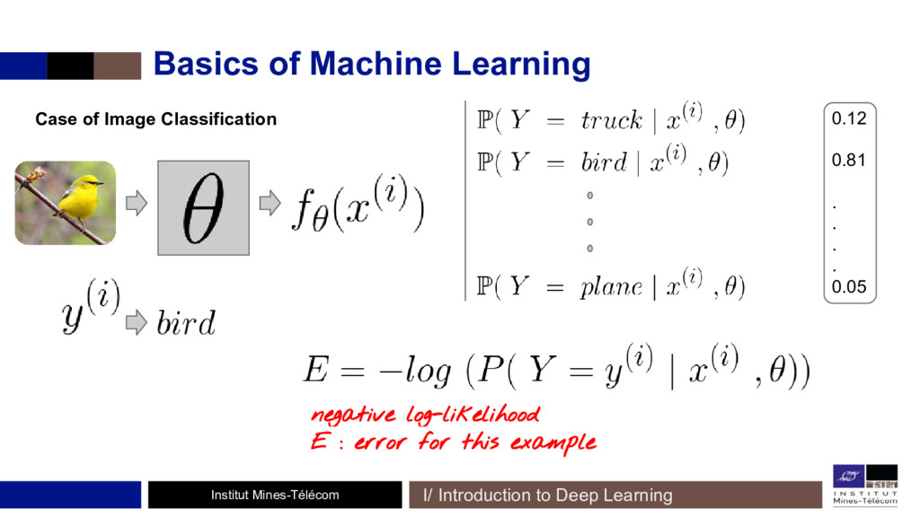
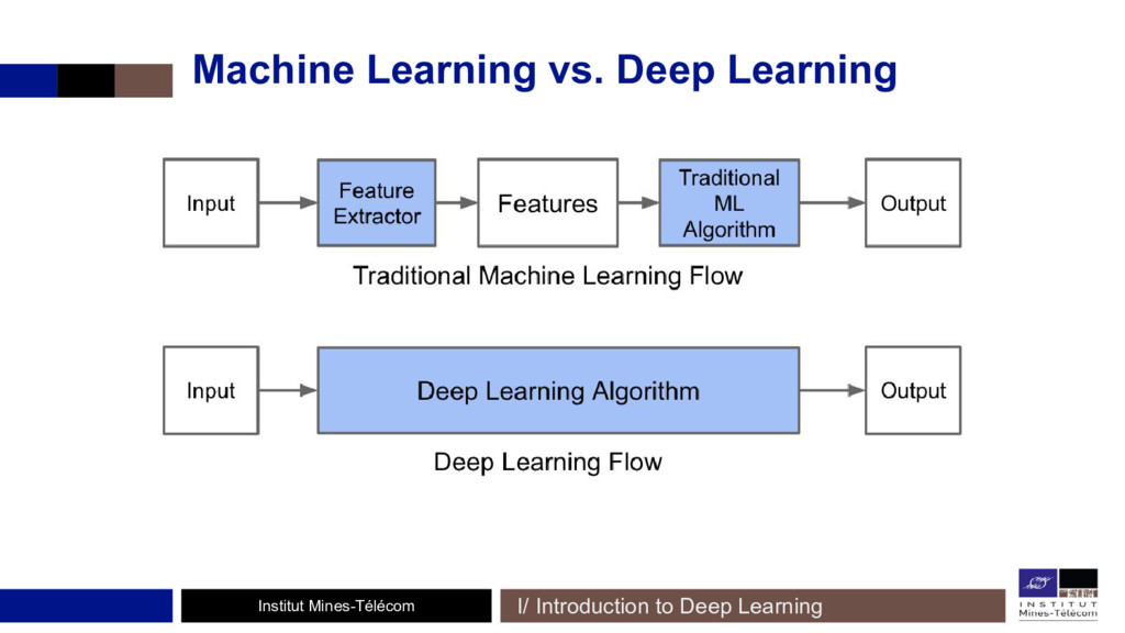
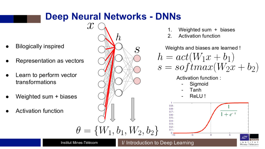
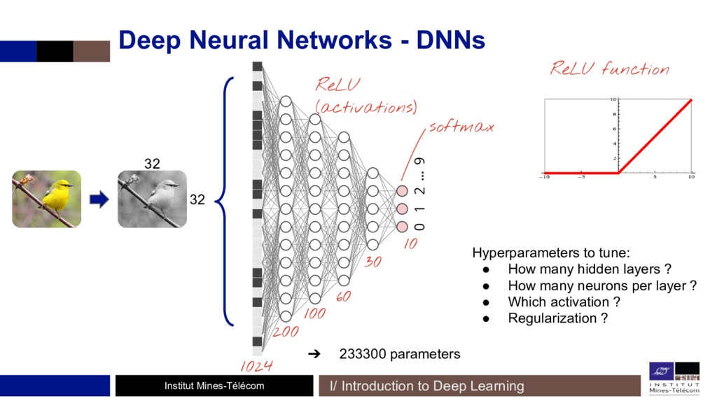
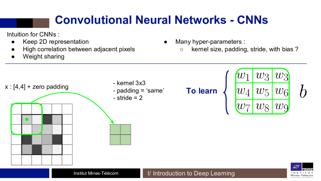
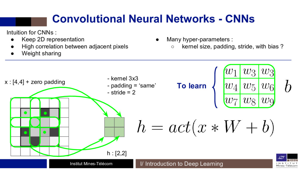
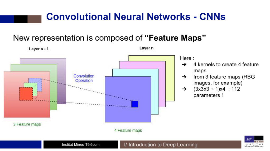
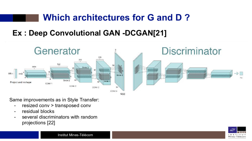
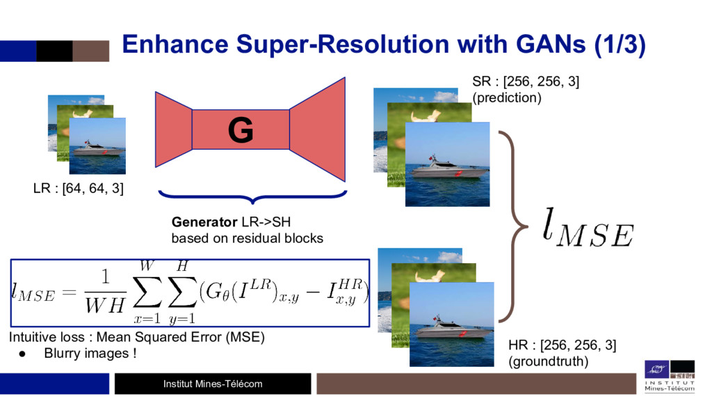
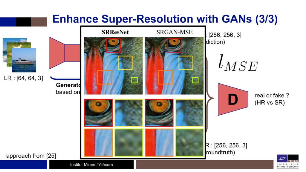
L'usage des GANs a permis d'obtenir de meilleurs résultats dans de nombreuses tâches où il est question de génération d'images: synthèse d'images, super-résolution, image-to-image translation, transfert de style, et beaucoup d'autres! Les GANs permettent aussi de faire du pré-apprentissage non-supervisé, pour obtenir de meilleurs résultats en classification d'images, même avec peu de données labellisées. En début de présentation, un rappel sera fait sur "Machine Learning vs Deep Learning" et les CNNs.

Bio : Julien Guillaumin est étudiant à Télécom Bretagne (Brest) en traitement d’images, Kaggler et MOOC friendly

Transcript

1. Institut Mines-Télécom
2. Institut Mines-Télécom TDS NoBlaBla : Style Transfer and Generative Adversarial Networks Julien Guillaumin julien.guillaumin@imt-atlantique.net IMT Atlantique (ex Télécom Bretagne)
3. Institut Mines-Télécom • Student at IMT Atlantique, Brest. ◦ Engineering degree - Computer Vision • Deep Learning Engineer at Lighton.io ◦ Optical co-processor for Machine Learning ◦ SummerIA.fr, Deep Learning Tutor ◦ Continental, Deep Learning for ADAS (intern) ◦ Thales Services, Large-scale Image Processing with Spark (intern) • Talks and MeetUps ◦ PyCon France 2016 ◦ Toulouse Data Science, Paris AI, Data Science Brest, Machine Learning Aix-Marseille ◦ Airbus Defence and Space, Quantmetry, Ercom
4. Institut Mines-Télécom Outline ▪ Introduction to Deep Learning • Basics of Machine Learning • Machine Learning vs Deep Learning • Convolutional Neural Networks - CNNs ▪ Style Transfer with Neural Networks • Perceptual loss : content loss + style loss • Optimization-based method: first steps in neural style transfer • Train CNNs to perform neural style transfer ▪ Generative Adversarial Networks - GANs • How to generate realistic images ? • Two networks, two players: Hi Game Theory ! • GANs for semi-supervised learning and domain adaptation • Can we understand the latent space ? • Applications: Super-resolution
5. Institut Mines-Télécom Introduction to Deep Learning
6. Institut Mines-Télécom Basics of Machine Learning ▪ Field of Artificial Intelligence ▪ Develop learnable algorithms • Learn from data • To resolve complex tasks ▪ Many tasks : • Natural Language Processing • Image classification • Object segmentation Two major phases : ▪ Training • From training data • Adjust internal parameters • Goal : find generalization ! ▪ Inference • New data (not seen) • Evaluation / Production I/ Introduction to Deep Learning
7. Institut Mines-Télécom Basics of Machine Learning 0.12 0.81 . . . . 0.05 negative log-likelihood E : error for this example Case of Image Classification I/ Introduction to Deep Learning
8. Institut Mines-Télécom Machine Learning vs. Deep Learning I/ Introduction to Deep Learning
9. Institut Mines-Télécom Machine Learning vs Deep Learning Random Forest ? (learned) Image space Feature space Output space Feature engineering (hand-designed) • Domain dependence • Need expert domain to tune • Hard to extract complex patterns For images : HOG features, SIFT methods, Histograms, LBP features, …. Machine Learning approach I/ Introduction to Deep Learning
10. Institut Mines-Télécom Machine Learning vs. Deep Learning SVM ? (learned) Image space Feature space Output space Learned feature extractor (learned) Representation Learning approach • Learn a new representation of the data • Ex : PCA (Principal Component Analysis) Logistic regression (learned) Image space Feature Space N Output space Deep Representation Learning approach • Learn a hierarchy of representations • Can be done with Neural Networks Feature Space 1 Feature Space 2 ... I/ Introduction to Deep Learning
11. Institut Mines-Télécom Deep Neural Networks - DNNs Activation function : - Sigmoid - Tanh - ReLU ! 1. Weighted sum + biases 2. Activation function Weights and biases are learned ! • Bilogically inspired • Representation as vectors • Learn to perform vector transformations • Weighted sum + biases • Activation function I/ Introduction to Deep Learning
12. Institut Mines-Télécom Deep Neural Networks - DNNs 9 ... 0 1 2 softmax 200 100 60 10 30 ReLU function 1024 ReLU (activations) 32 32 Hyperparameters to tune: • How many hidden layers ? • How many neurons per layer ? • Which activation ? • Regularization ? I/ Introduction to Deep Learning ➔ 233300 parameters
13. Institut Mines-Télécom Convolutional Neural Networks - CNNs Intuition for CNNs : • Keep 2D representation • High correlation between adjacent pixels • Weight sharing I/ Introduction to Deep Learning x : [4,4] + zero padding To learn - kernel 3x3 - padding = ‘same’ - stride = 2 • Many hyper-parameters : ◦ kernel size, padding, stride, with bias ?
14. Institut Mines-Télécom Convolutional Neural Networks - CNNs Intuition for CNNs : • Keep 2D representation • High correlation between adjacent pixels • Weight sharing I/ Introduction to Deep Learning x : [4,4] + zero padding - kernel 3x3 - padding = ‘same’ - stride = 2 • Many hyper-parameters : ◦ kernel size, padding, stride, with bias ? To learn h : [2,2]
15. Institut Mines-Télécom Convolutional Neural Networks - CNNs New representation is composed of “Feature Maps” Here : ➔ 4 kernels to create 4 feature maps ➔ from 3 feature maps (RBG images, for example) ➔ (3x3x3 + 1)x4 : 112 parameters ! I/ Introduction to Deep Learning
16. Institut Mines-Télécom Convolutional Neural Networks - CNNs Simple CNN : convolutional layers + DNNs ‘Flatten’ DNN Conv + activation Conv + activation I/ Introduction to Deep Learning Add pooling operations (Average, Max), to reduce the feature maps !
17. Institut Mines-Télécom Deep Network : VGG-16 [1] ▪ Simple : no inception modules[2] or residual connections[3] ▪ Trained for image classification on ImageNet[4] (1000 classes) ▪ State of the art in 2014 (92.7% top-5 test accuracy) ▪ 138,357,544 parameters (10% conv weights, 90% FC layers) 17 I/ Introduction to Deep Learning
18. Institut Mines-Télécom Neural Style Transfer
19. Institut Mines-Télécom Neural Style Transfer: Motivations II/ Neural Style Transfer ▪ Generative task • From an image, generate a new one ▪ Introduction to more complex tasks • Super-resolution and colorisation ▪ CNNs understanding is required • Hierarchy of representations • Feature spaces ? content image style image stylized image with content
20. Institut Mines-Télécom CNN visualization 20 Style Transfer - Visualizing and Understanding CNNs Convolution + ReLU Pooling conv5_3 (14x14x512) preprocessing conv1_1 (224x224x64) From low-level to high-level feature spaces Additional visualization methods : - Deep Dream approach [5] - Optimization-based - Zeiler & Fergus [6] - Transposed convolutions and unpooling operations core VGG-16 MLP - Classification
21. Institut Mines-Télécom Content Representation/Reconstruction 21 Fixed VGG-16 Style Transfer - Content & Style Representations conv3_3 : 56x56x256 Eg : : activations of the jth layer • Goal : find an image with the same activations at a given layer (all feature maps) • Optimization problem, start from a random image
22. Institut Mines-Télécom Content Representation/Reconstruction 22 Fixed VGG-16 • gradient descent optimization on input image, network does not change • loss = MSE on feature maps, 1000 iterations, Adam (lr=2.0) • low-level : input image is correctly reconstructed, with pixel-level details • high-level : only content is preserved Style Transfer - Content & Style Representations
23. Institut Mines-Télécom Content Representation/Reconstruction 23 Fixed VGG-16 Style Transfer - Content & Style Representations • From a random image, reconstruct the feature maps obtained with a normal image, on a specific layer • Gradient descent optimization on image input, network does not change • Loss = MSE on feature maps, 1000 iterations, Adam (lr=2.0) • Low-level : input image is correctly reconstructed, with pixel-level details • High-level : only content is preserved Content only
24. Institut Mines-Télécom Style Representation/Reconstruction 24 Style Transfer - Content & Style Representations • Needs more complex statistics on feature maps : Gram matrix ◦ Second-order statistics ◦ Can capture texture information, no spatial information • For a given layer j with feature maps of size • The Gram matrix is a matrix : • Where is an element-wise operation between 2 feature maps (Hadamard product) • Contains the correlation between every pair of feature maps
25. Institut Mines-Télécom Style Representation/Reconstruction 25 Style Transfer - Content & Style Representations Fixed VGG-16 conv3_3 : 56x56x256 Gram matrix of the jth layer (256 x 256) • Goal : To find an image with the same Gram matrix for a given layer • Optimization problem: Start from a random image
26. Institut Mines-Télécom Style Representation/Reconstruction 26 Fixed VGG-16 • Gradient descent optimization on image input, network is freezed • Loss = MSE on feature maps, 1000 iterations, Adam (lr=2.0) • Low-level : Small and simple patterns • High-level : More complex patterns Style Transfer - Content & Style Representations
27. Institut Mines-Télécom Content & Style Representations ▪ Content is preserved in high level features ▪ Style is present in second-order statistics in low and medium levels ▪ Content and Style are separable ▪ content_loss and a style_loss are defined ▪ Combine style and content from different images is possible, via feature extraction learned within a VGG network, trained on a generic image classification task ! 27 Style Transfer - Content & Style Representations
28. Institut Mines-Télécom Mix content & style via specific losses 28 Style Transfer - Optimization-based Style Transfer Pre-train VGG16 Euclidean distance on feature space (conv2_2) Weighted sum over euclidean distances between Gram matrices (con1_2, con2_2, conv3_3, conv4_3) Convolution + ReLU Pooling Perceptual loss and method defined in [7]
29. Institut Mines-Télécom Optimization process 29 Style Transfer - Optimization-based Style Transfer ▪ Compute content_target (feature maps) with content_image ▪ Compute style_target (Gram matrices) with style_image ▪ Start from a random image (input_image) ▪ Optimization process : • Compute content_loss and style_loss with targets + input_image • Minimize this loss by modifying input_image • Possible thanks to gradient-descent method (like Adam)
30. Institut Mines-Télécom TensorFlow implementation 30 Style Transfer - Optimization-based Style Transfer it = [100, 400, 800, 3000]
31. Institut Mines-Télécom Results ▪ Produce high-quality images ▪ Easy to tune effects (more content ? more style ?) ▪ Any input/output size ▪ Running time (1000 #iter) • GPU (GTX 1070) : ~ 5 min (1920 CUDA cores) • CPU (i7-7700K) : ~ 150 min (4 cores x 2 threads) ▪ Avoid any real-time applications ▪ But perceptual loss (content+style) is defined 31 Style Transfer - Optimization-based Style Transfer
32. Institut Mines-Télécom Improvements 32 Style Transfer - Optimization-based Style Transfer • Time dependency for video transformation (see [8]) • Change optimizer : L-BFGS ! • Tune weights between style and content loss • Start from : content image? style image? noisy image? or a mix? • Color constraint : preserve color from content image ! (see [9]) from : github.com/tensorflow/magenta
33. Institut Mines-Télécom Feed-forward method [10, 11] 33 Style Transfer - Feed-forward method • Train a network to obtain a stylized image in one pass as an output • Used for one specific style (fixed) Generator • Trained to add this style • With a dataset of content images • Same input/output size
34. Institut Mines-Télécom Architecture of the generator ? 34 Style Transfer - Feed-forward method Conv_block Conv layer IN layer ReLU Instance Normalization [11] Variant of Batch Normalization Residual_block Deconv_block (transposed conv) Transpose Conv IN layer ReLU Conv layer + tf.tanh() 3 feature maps 128 feature maps
35. Institut Mines-Télécom How to train a generator ? 35 Generator content image pre-trained VGG-16 style image • Train with batch of content images • Minimize total loss w.r.t. theta Style Transfer - Feed-forward method
36. Institut Mines-Télécom Need a dataset of content images 36 • COCO dataset[12], about 80k images • Only 1 style image Training process (loop) : • Take a batch of samples from COCO • Pass this batch through the generator to get generated images • Compute style_loss between the generated images and the style image • Compute content_loss between the generated images and the original ones • Minimize the total_loss by updating the weights from the generator Training information : • Adam optimizer (lr=0.05) • Only 20k iterations (with batch_size=4) • For 512x512x3: ◦ Training time (on GTX 1070) : 10 hours ◦ Inference time : 330 ms (GTX 1070) Style Transfer - Feed-forward method
37. Institut Mines-Télécom Results and improvements 37 • Learn to apply only one style (with fixed style/content levels!!) • In [13] (ICLR 2017) : ◦ Add ‘Conditional Instance Normalization’ ◦ Learn to apply a fixed set of styles (until 64) ◦ Can learn quickly a new style (incremental learning) • Use resized convolutions[14] instead of transposed convolutions : Improves quality • Add variational loss to encourage spatial smoothness • Now : Universal/Arbitrary Style Transfer ! [15, 16] • With a new content image : it = 500 it = 1 it = 20000 it = 2000 it = 12000 Style Transfer - Feed-forward method
38. Institut Mines-Télécom Conv vs. Transposed Conv Conv2d, kernel size : 3x3, stride=2, padding=’same’ x : [5, 5] , ẍ : [25,] y : [3,3], ÿ : [9,] M : [9, 25] y : [3, 3] , ŷ : [9,] TransposeConv2d, kernel size 3x3, stride=2, padding=”same ” Conv2d, kernel size 3x3, stride=1, “internal zero padding”, padding=”valid”, x : [5, 5] , x : [25,] More info about resized conv and transposed conv : https://distill.pub/2016/deconv-checkerboard/
39. Institut Mines-Télécom BatchNorm vs. InstanceNorm 39 Conv batch_size = 32 Activation [32, 128, 128, 3] [32, 64, 64, 5] [N, H, W, F] [32, 64, 64, 5] Normalization BatchNorm : channel-wise Discriminative tasks ! InstanceNorm : (sample,channel)-wise Generative tasks ! Style Transfer - Feed-forward method
40. Institut Mines-Télécom Conditional Instance Normalization : Add meta-data to your CNNs ! Add conditions on within an Instance Normalization layer : - Traffic Sign classification : - SAR images : [13] : Conditional Instance Normalization applied to Style Transfer - 64 styles with 1 generator and 64 sets of normalization parameters - direct interpolation with the learned normalization parameters to create new styles
41. Institut Mines-Télécom Some results
42. Institut Mines-Télécom Generative Adversarial Networks- GANs
43. Institut Mines-Télécom Some “generative” tasks Source :https://phillipi.github.io/pix2pix/ Paper [17]
44. Institut Mines-Télécom How to generate realistic images ? Task: given a dataset, generate samples following a distribution similar to the dataset Which loss to use ? - MSE (Mean Squared Error) on image space - Total Variation Loss (impose smoothness) - Feature Matching (MSE on feature maps) - Perceptual loss (cf Style Transfer) Blurred images, non-realistic images
45. Institut Mines-Télécom Find the Manifolds of ‘realistic images’ ? Ships vs Planes manifolds ! Main issue in Machine Learning : - How to define a good loss for a given task ?? MSE for image generation ? - Does not capture the concepts - Distance on low-level representation (pixel-level) ! Hard to define a loss that measure the photorealism ? LEARN THIS LOSS WITH NEURAL NETS
46. Institut Mines-Télécom How to generate cats : Meow generator ! ➔ start from a random noise ➔ to a realistic image in the manifold of cats ! ➔ with a ‘mapping’ function [100,] [256, 256, 3] (distributions) (samples)
47. Institut Mines-Télécom Generative Adversarial Networks (GANs) General framework : Generator(G) + Discriminator(D) - G : generates data from a latent space (noise) - D : is trained to classify real vs fake data - G : is trained to fool D G D “1” : Real data “0” : Fake data generated data training data (binary classification) Original paper [18]
48. Institut Mines-Télécom GANs in equations min/max game : Game Theory - 2 agents : 2 neural networks - equivalent to minimize the Jensen-Shannon divergence between - Nash equilibrium : - Learn an implicit distribution, throught the generator :
49. Institut Mines-Télécom In practice : how to train GANs ? Many other to train G and D : - f-divergence, Wasserstein loss, feature matching, .... see [19, 20](Jan 2018) Simultaneously training for D and G: - train G to fool D with a batch of z - train D to detect samples from G or from the dataset
50. Institut Mines-Télécom Which architectures for G and D ? Ex : Deep Convolutional GAN -DCGAN[21] Same improvements as in Style Transfer: - resized conv > transposed conv - residual blocks - several discriminators with random projections [22]
51. Institut Mines-Télécom Some results GAN, LapGAN, DCGAN, BeGAN, BiGAN, DiscoGAN, LSGAN, WGAN, f-GAN, Fisher-GAN, AE-GAN, APE-GAN, Gang of GANs, InfoGAN, CycleGAN, StackedGAN, DualGAN, DeliGAN, ….. -> Meow generator Here, results with a DCGAN, trained with `feature matching` loss !
52. Institut Mines-Télécom Latent Space understanding (z) Arithmetic operation in the latent space : How to get z from a photo : - recover z by optimization - learn an encoder z=E(x) when training D and G - BiGAN : GAN + auto-encoder [23]
53. Institut Mines-Télécom GANs for semi-supervised learning Unsupervised pre-training Supervised fine-training G D “1” : Real data “0” : Fake data generated data training data (unlabeled) (binary classification) D training data (labeled ! ) New part to train: task-specific classifier multi-class classifier !
54. Institut Mines-Télécom Adversarial Domain Adaptation (1/3) Target domain : MNIST ▪ without labels Source domain : SVHN ▪ with labels 60k + 10k samples 10 classes, 28x28 pixels ~ 150k samples 10 classes, 32x32 pixels Similar concepts, not the same data source (ex : optical vs SAR images)
55. Institut Mines-Télécom Adversarial Domain Adaptation (2/3) SVHN CNN Classifier Pre-training - supervised learning - on source domain - train ‘SVHN CNN’ + ‘Classifier’ SVHN CNN MNIST CNN Discriminator Task : binary classification - features ‘SVHN CNN’ - or from ‘MNIST CNN’ ? Adversarial Adaptation: - learn a target encoder CNN (Generator) - features from ‘MNIST CNN’ will follow the same distribution as the features from ‘SVHN CNN’ - without labels from both domains !
56. Institut Mines-Télécom Adversarial Domain Adaptation (3/3) MNIST CNN Classifier Testing - ‘Classifier’ can understand features from ‘MNIST CNN’ - and make classification Results : [24] : Adversarial Discriminative Domain Adaptation, E. Tzeng et al, Feb 2017
57. Institut Mines-Télécom Enhance Super-Resolution with GANs (1/3) LR : [64, 64, 3] HR : [256, 256, 3] (groundtruth) SR : [256, 256, 3] (prediction) Generator LR->SH based on residual blocks Intuitive loss : Mean Squared Error (MSE) • Blurry images ! G
58. Institut Mines-Télécom Enhance Super-Resolution with GANs (2/3) LR : [64, 64, 3] HR : [256, 256, 3] (groundtruth) SR : [256, 256, 3] (prediction) Generator LR->SH based on residual blocks G D real or fake ? (HR vs SR)
59. Institut Mines-Télécom Enhance Super-Resolution with GANs (3/3) LR : [64, 64, 3] HR : [256, 256, 3] (groundtruth) SR : [256, 256, 3] (prediction) Generator LR->SH based on residual blocks G D real or fake ? (HR vs SR) approach from [25]
60. Institut Mines-Télécom Many applications of GANs … Cross-domain image generation [26] (FAIR) paper [28] : “High-Resolution Image Synthesis and Semantic Manipulation with Conditional GANs”, Nvidia, Dec 2017 demo :https://www.youtube.com/watch?v=3AIpPlzM_qs Reverse style transfer with CycleGAN [27]
61. Institut Mines-Télécom Thanks !
62. Institut Mines-Télécom References (1/2) [1] : K. Simonyan, A. Zisserman : “Very Deep Convolutional Networks for Large-Scale Image Recognition”, 2014, arXiv:1409.1556 [2] : C Szegedy et al. : “Going Deeper with Convolutions”, 2014, arxiv:1409.4842 [3] : K He et al : “Deep Residual Learning for Image Recognition”, 2015, arxiv.org:1512.03385 [4] : ImageNet dataset : http://www.image-net.org/ [5] : About Deep Dream visualization technique : “Inceptionism: Going Deeper into Neural Networks” [6] : M. Zeiler, R. Fergus: Visualizing and Understanding Convolutional Networks, 2013 arXiv:1311.2901 [7] : L. Gatys, A. Ecker, M. Bethge : A neural algorithm of artistic style, 2015, arXiv:1508.06576 [8] : M. Ruder, A. Dosovitskiy, T. Brox : Artistic style transfer for video, 2016, arXiv:1604.08610 [9] : Gatys et al : Preserving color in Neural Artistic Style Transfer, 2016, arXiv:1606.05897 [10] : J. Johnson et al : “Perceptual losses for real-time style transfer and super-resolution”, 2016, arXiv:1603.08155 [11] : D. Ulyanov et al : “Instance Normalization: The Missing Ingredient for Fast Stylization”, 2016, arXiv:1607.08022 [12] : MS-COCO dataset : http://cocodataset.org/#home [13] : V. Dumoulin et al : “A learned representation for artistic style”, 2017, arXiv:1610.07629 [14] : A Aitken et al : “Checkerboard artifact free sub-pixel convolution”, 2017, arxiv.org:1707.02937 [15] : X. Huang and S. Belongie : “Arbitrary Style Transfer in real-time with AdaIN”, 2017, arXiv:1703.06868 [16] : Y Li et al : “Universal Style Transfer via Feature Transforms”, 2017, arxiv:1705.08086
63. Institut Mines-Télécom References (2/2) [17] : P Isola et al : “Image-to-Image Translation with Conditional Adversarial Networks”, 2016, arxiv:1611.07004 [18] : I Goodfellow et al : “Generative Adversarial Networks”, 2014, arxiv:1406.2661 [19] : Y Hong et al : “How GANs and its variants work : an overview of GAN”, 2017, arxiv:1711.05914v6 [20] : S Hitawala : “Comparative Study on GANs”, 2018, arxiv:1801.04271v1 [21] : A Radford et al : “Unsupervised Representation Learning with Deep Convolutional GANs”, 2015, arxiv:511.06434 [22] : B Neyshabur et al : “Stabilizing GAN Training with Multiple Random Projections”, 2017, arxiv:1707.02937 [23] : J Donahue et al : “Adversarial Feature Learning” , 2016, arxiv:1605.09782 [24] : Eric Tzeng et al : “Adversarial Discriminative Domain Adaptation”, 2017, arxiv:1702.05464 [25] : C Ledig et al : “Photo-realistic Single Image Super-Resolution using GANs” 2016, arxiv:1609.04802 [26] : Y Taigman et al : “Unsupervised Cross-Domain Image Generation”, 2016, arxiv:1611.02200 [27] : J-Y Zhu et al : “Unpaired Image-to-Image Translation using Cycle-Consistent Adversarial Networks”, 2017, arxiv:1703.10593 [28] : T-C Wang et al (NVIDIA) : “High-Resolution Image Synthesis and Semantic Manipulation with Conditional GANs”, Dec 2017, arxiv:1711.11585