Training Neural Networks at the Edge of Stability

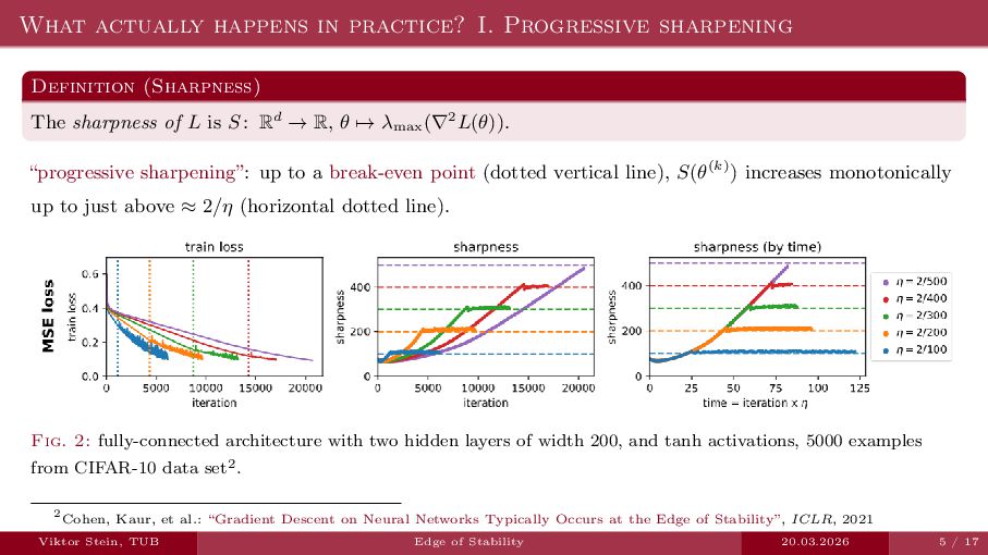
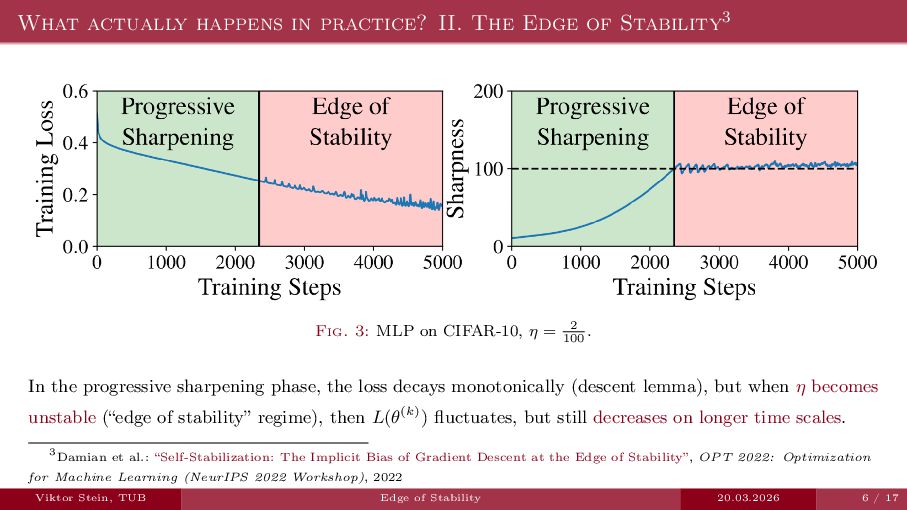
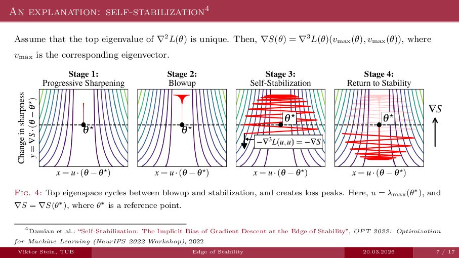
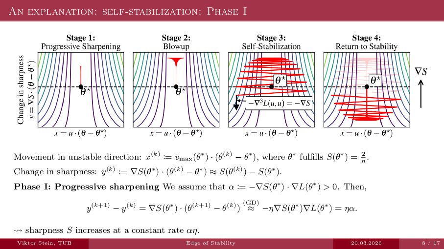
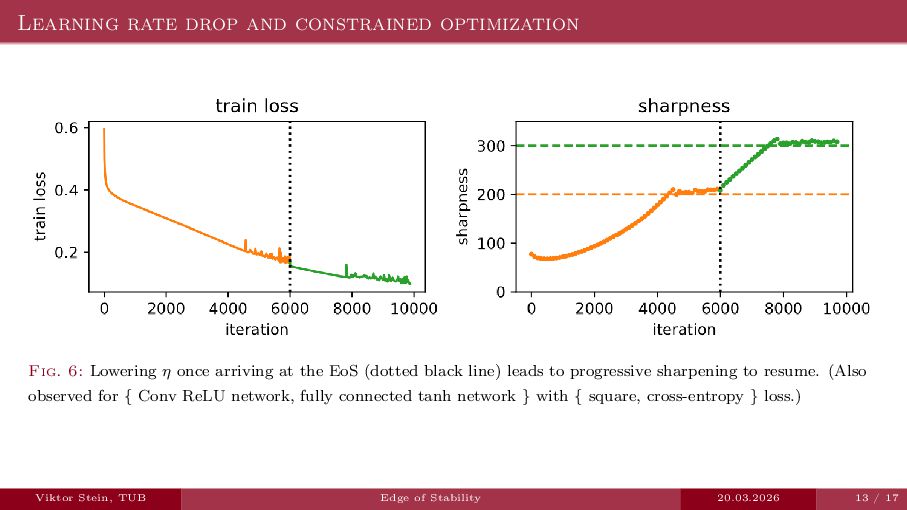
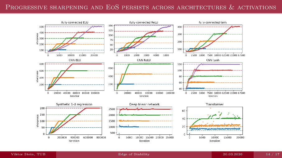
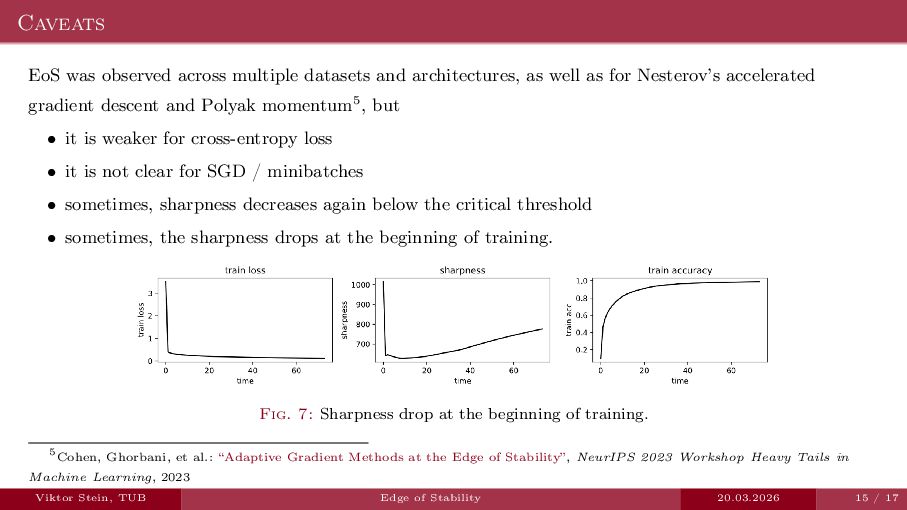
An expository talk about neural network training (progressive sharpening, edge of stability, self-stabilization) based on the two papers "Self-Stabilization: The Implicit Bias of Gradient Descent at the Edge of Stability" by Damian et al., and "Gradient descent on neural networks typically occurs at the edge of stability" by Cohen et la.

Transcript

1. Training Neural Networks at the Edge of Stability Viktor Stein, Technical University of Berlin Seminar: Mathematics of Machine Learning WiSe25/26 20.03.2026
2. 1. Two curious observations on gradient descent in neural network training 2. An explanation: self-stabilization 3. Caveats 4. Conclusions & future directions
3. Gradient-based optimization algorithms in machine learning Most neural network weights are optimized using Adam1 (or similar) on a loss L. 1Kingma and Ba: “Adam: A Method for Stochastic Optimization”, ICLR, 2015 Viktor Stein, TUB Edge of Stability 20.03.2026 3 / 17
4. Gradient-based optimization algorithms in machine learning Most neural network weights are optimized using Adam1 (or similar) on a loss L. 1Kingma and Ba: “Adam: A Method for Stochastic Optimization”, ICLR, 2015 Viktor Stein, TUB Edge of Stability 20.03.2026 3 / 17
5. Gradient-based optimization algorithms in machine learning Most neural network weights are optimized using Adam1 (or similar) on a loss L. Adam ≈ gradient descent + momentum + mini-batching + adaptive step sizes 1Kingma and Ba: “Adam: A Method for Stochastic Optimization”, ICLR, 2015 Viktor Stein, TUB Edge of Stability 20.03.2026 3 / 17
6. Gradient-based optimization algorithms in machine learning Most neural network weights are optimized using Adam1 (or similar) on a loss L. Adam ≈ gradient descent + momentum + mini-batching + adaptive step sizes Loss L is non-convex, so why does the neural network generalize well? 1Kingma and Ba: “Adam: A Method for Stochastic Optimization”, ICLR, 2015 Viktor Stein, TUB Edge of Stability 20.03.2026 3 / 17
7. Gradient-based optimization algorithms in machine learning Most neural network weights are optimized using Adam1 (or similar) on a loss L. Adam ≈ gradient descent Loss L is non-convex, so why does the neural network generalize well? We focus on plain gradient descent, supposing L ∈ C3(Rd): θ(k+1) = θ(k) − η∇L(θ(k)), θ(0) ∈ Rd, k ∈ N, η > 0. (GD) 1Kingma and Ba: “Adam: A Method for Stochastic Optimization”, ICLR, 2015 Viktor Stein, TUB Edge of Stability 20.03.2026 3 / 17
8. Gradient-based optimization algorithms in machine learning Most neural network weights are optimized using Adam1 (or similar) on a loss L. Adam ≈ gradient descent Loss L is non-convex, so why does the neural network generalize well? We focus on plain gradient descent, supposing L ∈ C3(Rd): θ(k+1) = θ(k) − η∇L(θ(k)), θ(0) ∈ Rd, k ∈ N, η > 0. (GD) Lemma (Descent lemma: decrease without convexity) If λmax (∇2L(θ)) ≤ ℓ for all θ ∈ Rd (“ℓ-smoothness”), then the gradient descent iterates fulfill L(θ(k+1)) ≤ L(θ(k)) − η 2 (2 − ηℓ)∥∇L(θ(k))∥2 2 , k ∈ N . 1Kingma and Ba: “Adam: A Method for Stochastic Optimization”, ICLR, 2015 Viktor Stein, TUB Edge of Stability 20.03.2026 3 / 17
9. Gradient-based optimization algorithms in machine learning Most neural network weights are optimized using Adam1 (or similar) on a loss L. Adam ≈ gradient descent Loss L is non-convex, so why does the neural network generalize well? We focus on plain gradient descent, supposing L ∈ C3(Rd): θ(k+1) = θ(k) − η∇L(θ(k)), θ(0) ∈ Rd, k ∈ N, η > 0. (GD) Lemma (Descent lemma: decrease without convexity) If λmax (∇2L(θ)) ≤ ℓ for all θ ∈ Rd (“ℓ-smoothness”), then the gradient descent iterates fulfill L(θ(k+1)) ≤ L(θ(k)) − η 2 (2 − ηℓ)∥∇L(θ(k))∥2 2 , k ∈ N . ⇝ choose η < 2 ℓ (“stable step size”), e.g. η = 1 ℓ , to ensure strictly monotone decrease of L 1Kingma and Ba: “Adam: A Method for Stochastic Optimization”, ICLR, 2015 Viktor Stein, TUB Edge of Stability 20.03.2026 3 / 17
10. Unstable step sizes Definition (Sharpness) The sharpness of L is S : Rd → R, θ → λmax (∇2L(θ)). Viktor Stein, TUB Edge of Stability 20.03.2026 4 / 17
11. Unstable step sizes Definition (Sharpness) The sharpness of L is S : Rd → R, θ → λmax (∇2L(θ)). For quadratic functions L, gradient descent resp. Polyak momentum resp. Nesterov’s accelerated gradient descent with momentum parameter β ∈ [0, 1] diverges if Viktor Stein, TUB Edge of Stability 20.03.2026 4 / 17
12. Unstable step sizes Definition (Sharpness) The sharpness of L is S : Rd → R, θ → λmax (∇2L(θ)). For quadratic functions L, gradient descent resp. Polyak momentum resp. Nesterov’s accelerated gradient descent with momentum parameter β ∈ [0, 1] diverges if S(θ) > 2 η resp. 2 η (1 + β) resp. 2 η 1 + β 1 + 2β . Viktor Stein, TUB Edge of Stability 20.03.2026 4 / 17
13. Unstable step sizes Definition (Sharpness) The sharpness of L is S : Rd → R, θ → λmax (∇2L(θ)). For quadratic functions L, gradient descent resp. Polyak momentum resp. Nesterov’s accelerated gradient descent with momentum parameter β ∈ [0, 1] diverges if S(θ) > 2 η resp. 2 η (1 + β) resp. 2 η 1 + β 1 + 2β . Fig. 1: With an unstable step size, gradient descent diverges, oscillating along top eigenvector (“unstable direction”). Viktor Stein, TUB Edge of Stability 20.03.2026 4 / 17
14. What actually happens in practice? I. Progressive sharpening Definition (Sharpness) The sharpness of L is S : Rd → R, θ → λmax (∇2L(θ)). “progressive sharpening”: up to a break-even point (dotted vertical line), S(θ(k)) increases monotonically up to just above ≈ 2/η (horizontal dotted line). Fig. 2: fully-connected architecture with two hidden layers of width 200, and tanh activations, 5000 examples from CIFAR-10 data set2. 2Cohen, Kaur, et al.: “Gradient Descent on Neural Networks Typically Occurs at the Edge of Stability”, ICLR, 2021 Viktor Stein, TUB Edge of Stability 20.03.2026 5 / 17
15. What actually happens in practice? II. The Edge of Stability3 Fig. 3: MLP on CIFAR-10, η = 2 100 . In the progressive sharpening phase, the loss decays monotonically (descent lemma), but when η becomes unstable (“edge of stability” regime), then L(θ(k)) fluctuates, but still decreases on longer time scales. 3Damian et al.: “Self-Stabilization: The Implicit Bias of Gradient Descent at the Edge of Stability”, OPT 2022: Optimization for Machine Learning (NeurIPS 2022 Workshop), 2022 Viktor Stein, TUB Edge of Stability 20.03.2026 6 / 17
16. An explanation: self-stabilization4 Assume that the top eigenvalue of ∇2L(θ) is unique. Then, ∇S(θ) = ∇3L(θ)(vmax (θ), vmax (θ)), where vmax is the corresponding eigenvector. Fig. 4: Top eigenspace cycles between blowup and stabilization, and creates loss peaks. Here, u = λmax(θ∗), and ∇S = ∇S(θ∗), where θ∗ is a reference point. 4Damian et al.: “Self-Stabilization: The Implicit Bias of Gradient Descent at the Edge of Stability”, OPT 2022: Optimization for Machine Learning (NeurIPS 2022 Workshop), 2022 Viktor Stein, TUB Edge of Stability 20.03.2026 7 / 17
17. An explanation: self-stabilization: Phase I Movement in unstable direction: x(k) := vmax (θ∗) · (θ(k) − θ∗), where θ∗ fulfills S(θ∗) = 2 η . Change in sharpness: y(k) := ∇S(θ∗) · (θ(k) − θ∗) ≈ S(θ(k)) − S(θ∗). Phase I: Progressive sharpening We assume that α := −∇S(θ∗) · ∇L(θ∗) > 0. Then, y(k+1) − y(k) = ∇S(θ∗) · (θ(k+1) − θ(k)) (GD) ≈ −η∇S(θ∗)∇L(θ∗) = ηα. ⇝ sharpness S increases at a constant rate αη. Viktor Stein, TUB Edge of Stability 20.03.2026 8 / 17
18. An explanation: self-stabilization: Phase II Movement in unstable direction: x(k) := vmax (θ∗) · (θ(k) − θ∗), where θ∗ fulfills S(θ∗) = 2 η . Change in sharpness: y(k) := ∇S(θ∗) · (θ(k) − θ∗) ≈ S(θ(k)) − S(θ∗). Phase II: Blowup We have ∇L(θ(k)) ≈ S(θ(k)) · (θ(k) − θ∗) because |x(k)| is small. Thus, x(k+1) (GD) = x(k) −ηvmax (θ∗)·∇L(θ(k)) ≈ x(k) −ηS(θ(k))x(k) ≈ x(k) −η 2 η + y(k) x(k) = −(1−ηy(k))x(k). ⇝ when S(θ(k)) > 2/η (i.e. y(k) > 0), then (|xt |)t∈N grows exponentially. Viktor Stein, TUB Edge of Stability 20.03.2026 9 / 17
19. An explanation: self-stabilization: Phase III Movement in unstable direction: x(k) := vmax (θ∗) · (θ(k) − θ∗), where θ∗ fulfills S(θ∗) = 2 η . Change in sharpness: y(k) := ∇S(θ∗) · (θ(k) − θ∗) ≈ S(θ(k)) − S(θ∗). Phase III: Self-stabilization y(k+1) − y(k) (GD) ≈ ηα + ∇S(θ∗) · −η∇3L(vmax (θ∗), vmax (θ∗)) (x(k))2 2 = η α − ∥∇S(θ∗)∥ (x(k))2 2 . ⇝ once x(k) > 2α ∥∇S(θ∗)∥ , sharpness decreases until it dips below 2 η . Viktor Stein, TUB Edge of Stability 20.03.2026 10 / 17
20. An explanation: self-stabilization: Phase IV Movement in unstable direction: x(k) := vmax (θ∗) · (θ(k) − θ∗), where θ∗ fulfills S(θ∗) = 2 η . Change in sharpness: y(k) := ∇S(θ∗) · (θ(k) − θ∗) ≈ S(θ(k)) − S(θ∗). Phase IV: Return to stability Again, y(k+1) − y(k) (GD) ≈ −(1 − ηy(k))x(k). ⇝ since now y(k) < 0, |x(k)| shrinks expoentially =⇒ back to phase I. Viktor Stein, TUB Edge of Stability 20.03.2026 11 / 17
21. Empirical verification Fig. 5: Gradient is unstable for unstable step sizes. The gradient descent iterates θ(k) follow closely the iterations of ˜ θ(k+1) := projM (˜ θ(k) − η∇L(˜ θ(k))), where M := {θ ∈ Rd : S(θ) < 2/η, ∇L(θ)vmax (θ) = 0}. Viktor Stein, TUB Edge of Stability 20.03.2026 12 / 17
22. Learning rate drop and constrained optimization Fig. 6: Lowering η once arriving at the EoS (dotted black line) leads to progressive sharpening to resume. (Also observed for { Conv ReLU network, fully connected tanh network } with { square, cross-entropy } loss.) Viktor Stein, TUB Edge of Stability 20.03.2026 13 / 17
23. Progressive sharpening and EoS persists across architectures & activations Viktor Stein, TUB Edge of Stability 20.03.2026 14 / 17
24. Caveats EoS was observed across multiple datasets and architectures, as well as for Nesterov’s accelerated gradient descent and Polyak momentum5, but • it is weaker for cross-entropy loss • it is not clear for SGD / minibatches • sometimes, sharpness decreases again below the critical threshold • sometimes, the sharpness drops at the beginning of training. Fig. 7: Sharpness drop at the beginning of training. 5Cohen, Ghorbani, et al.: “Adaptive Gradient Methods at the Edge of Stability”, NeurIPS 2023 Workshop Heavy Tails in Machine Learning, 2023 Viktor Stein, TUB Edge of Stability 20.03.2026 15 / 17
25. Conclusion & further directions Conclusion • Standard optimization heuristics like η < 2/ℓ do not explain neural network training • progressive sharpening up to the break-even point, then edge of stability • self-stabilization explains hovering over critical rate Further directions • non-heuristic proofs for small settings6 • Good explanation of SGD behavior (which quantities to track?) • Explain why Adam or RMSprop work well 6Yoo et al.: “Understanding Sharpness Dynamics in NN Training with a Minimalist Example: The Effects of Dataset Difficulty, Depth, Stochasticity, and More”, Forty-second International Conference on Machine Learning, 2025 Viktor Stein, TUB Edge of Stability 20.03.2026 16 / 17
26. Thank you for your attention! I am happy to take any questions. Viktor Stein, TUB Edge of Stability 20.03.2026 17 / 17
27. Bibliography [1] D. Kingma and J. Ba, “Adam: A method for stochastic optimization,” in ICLR, Dec. 2015. [2] J. Cohen, S. Kaur, Y. Li, J. Z. Kolter, and A. Talwalkar, “Gradient descent on neural networks typically occurs at the edge of stability,” in ICLR, 2021. [3] A. Damian, E. Nichani, and J. D. Lee, “Self-stabilization: The implicit bias of gradient descent at the edge of stability,” in OPT 2022: Optimization for Machine Learning (NeurIPS 2022 Workshop), 2022. [4] J. Cohen, B. Ghorbani, et al., “Adaptive gradient methods at the edge of stability,” in NeurIPS 2023 Workshop Heavy Tails in Machine Learning, 2023. [5] G. Yoo, M. Song, and C. Yun, “Understanding sharpness dynamics in nn training with a minimalist example: The effects of dataset difficulty, depth, stochasticity, and more,” in Forty-second International Conference on Machine Learning, 2025. Viktor Stein, TUB Edge of Stability 20.03.2026 1 / 1