Separation of Bounded Arithmetic using a consistency statement

Transcript

1. Separation of bounded arithmetic using a consistency statement SLACS 2019, Kyoto University Yoriyuki Yamagata AIST, Japan Sep. 9, 2019
2. This presentation about ... A possible proof strategy of Separation of Buss’s S1 2 and S2, S1 2 S2 (?) As a corollary, P = NP (?!) I do not believe it at all, but it may contain interesting techniques or conjectures Draft: https://www.dropbox.com/s/g22x84rfdqmyx82/
3. Draft and slides location Figure: Draft location Figure: Slides location
4. Definition of Buss’s Si 2 [Buss, 1986] Si 2 is formulated by PIND for Σb i -formula plus axioms Ax. 1 Ax is finite, 2 all formulas in Ax are true in the standard interpretation, 3 all formulas in Ax is quantifier free, 4 Ax implies all BASICe axioms in [Buss and Ignjatovi´ c, 1995] 5 Ax implies formulas corresponding P = NP in [Takeuti, 1996] if P = NP. S2 := i=1,2,... Si 2
5. Definition of Cook’s PV [Cook, 1975] 1 Defining axioms for polynomial-time functions 2 Identity axioms 3 Substitution axiom 4 Induction axiom Consistency of (1) and (2) inside S1 2 is proven in [Beckmann, 2002] Consistency of (1) - (3) inside S2 2 is proven in [Yamagata, 2018] Definition PV− is a system obtained from PV by dropping induction axiom PV− 1 = PV− + first order logic PV− 1 (D) is the restriction of PV− 1 in which the number of quantifiers and equations is bounded by D.
6. Proof strategies 1 Define PV− q (D), an extension of PV− with finite number D of Henkin-like quantifiers 2 Prove consistency of PV− q (D) in S2 3 Embed PV− 1 (D) to PV− q (D) in S2 4 Prove embedded PV− 1 (D) + Ax is consistent in S2 5 Prove consistency of PV− 1 (D) + Ax is not provable in S1 2 5. is modification of [Buss and Ignjatovi´ c, 1995] Our tasks are 1-4
7. Dependency matrix Definition A dependency matrix Q is a sequence of 1 x(x1, . . . , xn) 2 {x}(x1, . . . , xn) in which all x are different (but x1, . . . , xn may have overlap) x(x1, . . . , xn) is a existential quantification which depends on x1, . . . , xn {x}(x1, . . . , xn) is a universal quantification which depends on x1, . . . , xn A dependency matrix is almost like a Henkin quantifier [Krynicki and Mostowski, 1995], but the order has meaning (to construct a semantics)
8. Language and proofs of PV− q (D) Definition Language of S2 plus Boolean variables and terms Additional functions bit(x, y): |y|-th bit of x p is the if-then-else function p(⊥, x, y) = x and p( , x, y) = y Boolean functions !, &, ||, →, ↔ A formula of PV− q is a form Q =⇒ φ where Q is a dependency matrix and φ is an equation Definition PV− q (D)-proofs are tree of PV− q (D)-formulas built by the following axioms and rules
9. Axioms All defining axioms for polynomial-time functions plus bit(ε, xW) = ⊥ bit(0xW, ε) = ⊥ bit(1xW, ε) = bit(bx, b y) = bit(x, y) p(⊥, x, y) = x p( , x, y) = y Finite many axioms of Boolean algebra t(x1, . . . , xn) = u(x1, . . . , xn)
10. Inference: quantifier reordering Q1, x(x), y([x, ]y), Q2 =⇒ φ Q1, y([x, ]y), x(x), Q2 =⇒ φ Q1, {x}(x), {y}([x, ]y), Q2 =⇒ φ Q1, {y}([x, ]y), {x}(x), Q2 =⇒ φ Q1, x(x), {y}(y), Q2 =⇒ φ Q1, {y}(y), x(x), Q2 =⇒ φ Q1, {x}(x), y(y), Q2 =⇒ φ Q1, y(y), {x}(x), Q2 =⇒ φ where y ∈ {x} and x ∈ {y} and [. . .] means it is optional
11. Inference: removing unused quantification Q1, x(y), Q2 =⇒ φ Q1, Q2 =⇒ φ Q1, {x}(y), Q2 =⇒ φ Q1, Q2 =⇒ φ if x is not a free variable in Q2 =⇒ φ
12. Inference: introduction and elimination of quantifiers Q =⇒ φ(y) {y}(y), Q =⇒ φ(y) Q =⇒ φ(t) Q, x(FV(t)) =⇒ φ(x) if y is not a bound variable of Q and y is a free variables of Q =⇒ φ(y) Q1, {x}(x) =⇒ φ(x) Q1 =⇒ φ(t) if FV(t) ⊆ {x}
13. Inference: axioms and equality rules Q1 =⇒ φ for axiom φ Q1 =⇒ u = t Q1 =⇒ t = u Q1 =⇒ t = u Q2 =⇒ u = r Q1, Q2 =⇒ t = r u if Q1, Q2 is a well-formed dependency matrix
14. Inference: compatibility of equality and p-rule Q1 =⇒ t1 = u1 · · · Qn =⇒ tn = un Q1, . . . , Qn =⇒ f (t1, . . . , tn) = f (u1, . . . , un) Q1 =⇒ t1 = u1 Q2 =⇒ t2 = u2 Q1, Q2 =⇒ p(b, t1, t2) = p(b, u1, u2)
15. A computation: idea A PV− q -proof of . . . . Q =⇒ t = u is interpreted as a constraction of a “computation” of ξ(u) from a “computation” of ξ(t) and reverse direction, where quantifiers Q is interpreted by substitutions ξ
16. A computation: problem I Problem I The size of a computation can be exponential, e.g. 2#2#2# · · · #2 Therefore, the proof cannot construct a computation of the lefthand from the righthand proj1 2 (0, 2#2#2# · · · #2) = 0 Solution Introduce unknown value ∗
17. A computation: problem II Problem What is the value of bit(∗, ∗)? We want to interpret the value of a Boolean term as a real Boolean, not, for example, a three-valued logic, so that we can prove that ⊥ = is never derived Solution We choose the value of bit(∗, ∗) randomly, yet consistently across the same computation. For this purpose, we incorporate the evaluation of bit(∗, ∗) into an evaluation environment ρ
18. Approximate value: g-numerals Definition ([Beckmann, 2002, Yamagata, 2018]) g-numerals v ∈ W := ε | ∗ | 0v | 1v Approximate relation is defined as: ε ε, v ∗, v w =⇒ bv bw for b = 0, 1, If v w then w is often written as v∗. G-numerals and Boolean values are called g-values
19. A environment and computation statement Definition An environment ρ of t is a map uW → v ∈ W uB → b ∈ B = {⊥, } for subformulas of t t ∈ dom(ρ) ⇐⇒ ρ(t) is defined. Definition A computational statement is a form t, ρ ↓ v where t is a term, ρ is an environment and v is a g-value.
20. Computation rules I Computations are DAGs built by the following rules: tW, ρ ↓ ∗ ∗ x, ρ ↓ v∗ Env where v = ρ(x) v, ρ ↓ v∗ v where v is a numeral t, ρ ↓ v bt, ρ+ ↓ bv∗ b where b is either 0 or 1 and t is not a numeral.
21. Computation rules II ( ti , ρ ↓ vi )i=1,...,m εm(t1, . . . , tm), ρ+ ↓ ε εm ( tj , ρ ↓ vj )j=1,...,m proji m (t1, . . . , tm), ρ+ ↓ v∗ i proji m t, ρ ↓ ⊥ u1, ρ ↓ v1 u2, ρ ↓ v2 p(⊥, u1, u2), ρ+ ↓ v∗ 1 p t, ρ ↓ u1, ρ ↓ v1 u2, ρ ↓ v2 p( , u1, u2), ρ+ ↓ v∗ 2 p
22. Computation rules III t, ρ ↓ v u, ρ ↓ w bit(t, u), ρ ↓ b bit where b is determined by bit(ε, w) = ⊥ if w = ∗ bit(bv, ε) = b bit(bv, b w) = bit(v, w). If bit(v, w) function is undefined, we often write bit(v, w) = ∗. If bit(v, w) = ∗, we put b = ρ(bit(t, u)).
23. Computation rules IV For Boolean connectives t, ρ ↓ b !t, ρ ↓ !b ! t1, ρ ↓ b1 t2, ρ ↓ b2 t1&t2, ρ ↓ b1&b2 & ⊥, ρ ↓ ⊥ ⊥ , ρ ↓ If f is defined by composition, we have the following rule. g(y, ξ ↓ z h1(x), ν ↓ w1 · · · hm(x), ν ↓ wm ( ti , ρ ↓ vi )i=1,...,n f (t1, . . . , tn), ρ+ ↓ z∗ where y = y1, . . . , ym, x = x1, . . . , xn, ν(xi ) = vi , i = 1, . . . , n and ξ(yj ) = wj , j = 1, . . . , m.
24. Computation rules V If f is defined by recursion, we have the following rules. gε(x1, . . . , xn), ξ ↓ z t, ρ ↓ ε ( ti , ρ ↓ vi )i=1,...,n f (t, t1, . . . , tn), ρ+ ↓ z∗ rec-ε where ξ(xi ) = vi for i = 1, . . . , n. gb(x0, y, x), ξ ↓ z t, ρ ↓ bv0 f (x0, x), ν ↓ w ( tj , ρ ↓ vj )j=1,...,n f (t, t1, . . . , tn), ρ+ ↓ z∗ where b = 0, 1 and x = x1, . . . , xn. The environment ν is defined by ν(xj ) = vj for j = 1, . . . , n and ν(x0) = v0 while ξ is defined by ξ(xj ) = vj , ξ(x0) = v0, ξ(y) = w.
25. Complexity of computations Definition For a computation σ, C(σ) is the minimum value which satisfies nodes(σ) ≤ C(σ) size(t) ≤ C(σ) if t, ρ ↓ v ∈ σ nodes(v) ≤ C(σ) if t, ρ ↓ v ∈ σ
26. Basic properties - computation of successors Lemma (S1 2 ) If ε, ρ ↓ v is contained in a computation σ, then either v ≡ ε or v ≡ ∗. If bt, ρ ↓ v where t is not a numeral, is contained in σ, then either v ≡ bv0 for some g-value v0 or v ≡ ∗. If v ≡ bv0, then σ contains t, ρ∗ ↓ v0 and v0 v0. Proof. Induction on σ
27. Basic properties - computation of numerals Lemma (S1 2 ) If v, ρ ↓ w, in which v are a numeral, is contained in a computation σ, then v w. Proof. Only rules which can derive v, ρ ↓ w are ∗ and v-rules.
28. Maximal environment Definition (maximal environment) For an environment ρ and a term of type W, we define V (t, ρ) = {v | σ t, ρ ↓ v, C(σ) ≤ nodes(t) · U} vals(t, ρ) = {v ∈ V (t, ρ) | v ∈ V (t, ρ), v v =⇒ v = v} ρ is maximal if ρ(t) ∈ vals(t, ξ) and ρ(bit(a, b)) = bit(ρ(a), ρ(b)) if bit(ρ(a), ρ(b)) = ∗. Env(ρ, t, U) ⇐⇒ ρ is a maximal environment . Env(ρ, t, U) is a bounded formula.
29. Substitution into ρ Lemma Let ρ be a maximal environment. Then, there is a maximal environment ρ such that ρ (x) = ρ(u) ρ(t(u)) ρ (t(x))
30. Basic properties - compatibility lemma Definition is defined as v w ⇐⇒ either v w or w v ρ1 ρ2 ⇐⇒ ρ1(t) ρ2(t) for any t ∈ dom(ρ1) ∩ dom(ρ2) For Boolean b1, b2, define b1 b2 ⇐⇒ b1 = b2 Lemma (S2: Compatibility lemma) Let ρ1 and ρ2 be maximal environments which satisfy ρ1 ρ2, t be the term. If both of t, ρ1 ↓ v and t, ρ2 ↓ w are contained in computations σ and τ respectively, then v w.
31. Most accurate evaluation in σ Definition Compatibility lemma allows extracting the most “accurate” value v(t, ρ, σ) of t evaluated in a maximal environment ρ from a computation
32. Basic properties - substitution lemma I Lemma (S2, Substitution Lemma I) Let ρ, ρ be maximal environments ρ is an extension of ρ ρ (xi ) = wi ρ (bit(r(x), s(x))) = ρ(bit(r(u), s(u))) σ t1(u1, . . . , un), ρ ↓ v1, . . . , tm(u1, . . . , un), ρ ↓ vm. =⇒ ∃τ t1(x), ρ ↓ v1, . . . , tm(x), ρ ↓ vm. s.t. C(τ) ∈ C(σ) + m j=1 size(tj (ε, . . . , ε))
33. Basic properties - substitution lemma II Lemma (S2, Substitution Lemma II) Let ρ, ρ be maximal environments s.t. ρ is an extension of ρ ρ (xi ) = wi ρ (bit(r(x), s(x))) = ρ(bit(r(u), s(u))) σ t1(x1, . . . , xn), ρ ↓ v1, . . . , tm(x1, . . . , xn), ρ ↓ vm =⇒ ∃τ t1(u1, . . . , un), ρ ↓ v1, . . . , tm(u1, . . . , un), ρ ↓ vm s.t. C(τ) ≤ max(C(σ) + m j=1 size(tj (ε, . . . , ε)), M(τ)).
34. Basic properties - defining and Boolean axioms Lemma t = u : substitution instance of an axiom σ t, ρ ↓ v, α =⇒ ∃τ u, ρ ↓ v, α s.t. C(τ) ≤ C(σ) + size(t = u)
35. Consistency proof - preliminaries Definition [q1/x1] · · · [qd /xd ], d ≤ D is called substitution sequence if x1, . . . , xd are all different dom(ξ) = {x1, . . . , xd } ξ(t) ≡ t[qd /xd ] · · · [q1/x1] B(ξ) = max{size(ξ(xi )) | i = 1, . . . , d} ξ : η is the concatenation of ξ and η Env(ρ, t, U): ρ is a maximal environment or t. U is the same U in the definittion of maximal environments.
36. Consistency proof - Sat relation for equality Definition U, B be integers such that U ≥ 2B ρ a maximal environment α judgements ξ be a substitution sequence such that B(ξ) ≤ (U − B)d Sat(U, B, ξ, ρ, α, t = u) ⇐⇒ ∀σ ξ(t), ρ ↓ v, α s.t. C(σ) ≤ (U − B)D+2, ∃τ ξ(u), ρ ↓ v, α s.t. C(τ) ≤ C(σ) + BD+2 and the ymmetric clause
37. Consistency proof - Sat relation for quantifiers Definition For universal, Sat(U, B, ξ, ρ, α, {x}(z1, . . . , zm), Γ =⇒ φ) ⇐⇒ ∀q, B([q/x] : ξ) ≤ (U − B)d , s.t. FV(q) ⊆ {z1, . . . , zm}, Sat(U, B, [q/x] : ξ, ρ, α, Γ =⇒ φ) For existential, Sat(U, B, ξ, ρ, α, x(z1, . . . , zm), Γ =⇒ φ) ⇐⇒ B ≤ ∀B ≤ U/2, ∃q, B([q/x] : ξ) ≤ (U − B )d s.t. FV(q) ⊆ {z1, . . . , zm}, Sat(U, B , [q/x] : ξ, ρ, α, Γ =⇒ φ)
38. Consistency proof - properties of Sat Lemma (S2, monotonicity) If B1 ≤ B2, Sat(U, B1, ξ, ρ, α, S) =⇒ Sat(U, B2, ξ, ρ, α, S) Lemma (S2, substitution for Sat) Let p be a term such that ξ(q) = q. ∀ρ, Env(ρ, UD+2) → Sat(U, B, ξ, ρ, α, t(x) = u(x)) =⇒ ∀ρ, Env(ρ, UD+2) → Sat(U, B + size(t(ε) = u(ε)), ξ, ρ, α, t(q) = u(q))
39. Consistency proof - soundness theorem Theorem (S2, soundness) a proof χ of PV− q (D) of S ≡ Q =⇒ φ an integer U s.t. U ≥ 2size(χ) a substitution sequence η ≡ [q1/x1] · · · [qd /xd ] s.t. B(η) ≤ (U − size(χ))d a sequence of statements α s.t. M(α) ≤ (U − size(χ))D+2 where M(α) is the maximum size of terms appearing in α. Then, Sat(U, size(χ), η, ρ, α, S) holds.
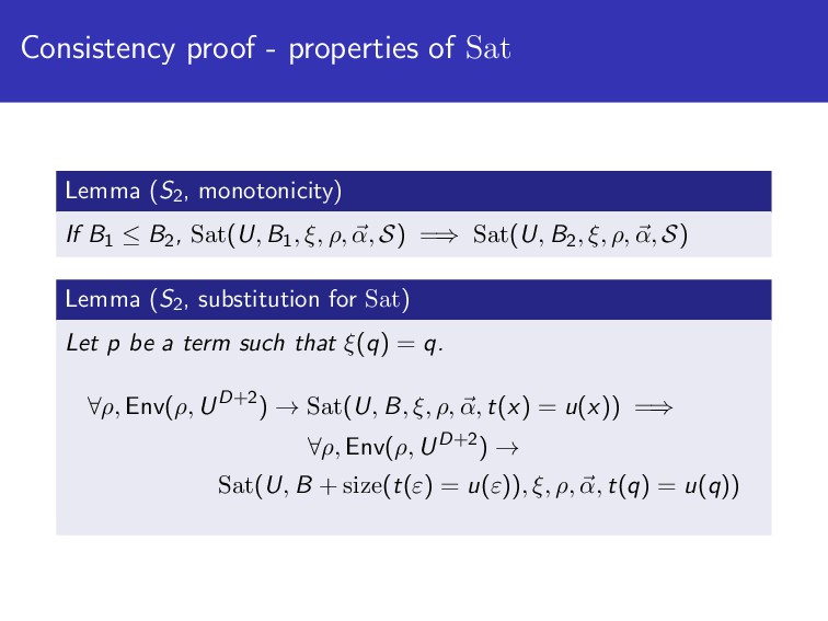
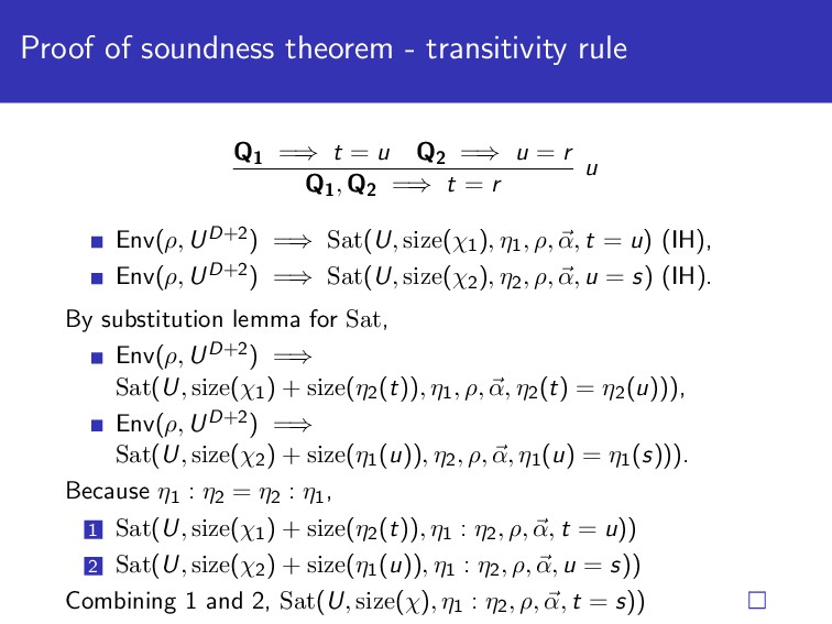
40. Proof of soundness theorem - transitivity rule Q1 =⇒ t = u Q2 =⇒ u = r Q1, Q2 =⇒ t = r u Env(ρ, UD+2) =⇒ Sat(U, size(χ1), η1, ρ, α, t = u) (IH), Env(ρ, UD+2) =⇒ Sat(U, size(χ2), η2, ρ, α, u = s) (IH). By substitution lemma for Sat, Env(ρ, UD+2) =⇒ Sat(U, size(χ1) + size(η2(t)), η1, ρ, α, η2(t) = η2(u))), Env(ρ, UD+2) =⇒ Sat(U, size(χ2) + size(η1(u)), η2, ρ, α, η1(u) = η1(s))). Because η1 : η2 = η2 : η1, 1 Sat(U, size(χ1) + size(η2(t)), η1 : η2, ρ, α, t = u)) 2 Sat(U, size(χ2) + size(η1(u)), η1 : η2, ρ, α, u = s)) Combining 1 and 2, Sat(U, size(χ), η1 : η2, ρ, α, t = s))
41. Proof of soundness theorem - universal quantification Q =⇒ t(x) = u(x) {x}(x), Q =⇒ t(x) = u(x) For q, B([q/x] : ξ) ≤ (U − size(χ))d+1 s.t. FV(q) ⊆ {x}. By induction hypothesis, ∀ρ, Env(UD+2, ρ) → Sat(U, B, ξ, ρ, α, t(x) = u(x)) By substitution Sat(U, size(χ1) + size(t(ε) = u(ε)), ξ, ρ, α, t(q) = u(q)) Therefore, Sat(U, size(χ), [q/x] : ξ, ρ, α, t(x) = u(x))
42. PV1 - axioms A PV1-proof is a tree of sequents built by following axioms and rules. The subsystem PV1(D) is a system in which for all sequents Γ =⇒ ∆, the number of quantifiers plus the number of equations is bounded by D. t = u =⇒ t = u =⇒ t = t t = u =⇒ u = t t = u, u = s =⇒ t = s t1 = u1, . . . , tm = um =⇒ f (t1, . . . , tm) = f (u1, . . . , um) if f (x1, . . . , xm) = t is a defining axiom, =⇒ f (u1, . . . , um) = t(u1, . . . , um)
43. PV1 - structural and propositional rules Γ =⇒ ∆ φ, Γ =⇒ ∆ Γ =⇒ ∆ Γ =⇒ ∆, φ φ, φ, Γ =⇒ ∆ φ, Γ =⇒ ∆ Γ =⇒ ∆, φ, φ Γ =⇒ ∆, φ φi , Γ =⇒ ∆ φ1 ∧ φ2, Γ =⇒ ∆ (i = 1, 2) Γ =⇒ ∆, φ1 Σ =⇒ Π, φ2 Γ, Σ =⇒ ∆, Π, φ1 ∧ φ2 Γ =⇒ ∆, φ ¬φ, Γ =⇒ ∆ φ, Γ =⇒ ∆ Γ =⇒ ∆, ¬φ
44. PV1 - predicate and cut rules φ(t), Γ =⇒ ∆ ∀x.φ(x), Γ =⇒ ∆ Γ =⇒ ∆, φ(x) Γ =⇒ ∆, ∀x.φ(x) if x ∈ FV(Γ, ∆) φ(x), Γ =⇒ ∆ ∃x.φ(x), Γ =⇒ ∆ if x ∈ FV(Γ, ∆) Γ =⇒ ∆, φ(t) Γ =⇒ ∆, ∃x.φ(x) Γ =⇒ ∆, φ φ, Σ =⇒ Π Γ, Σ =⇒ ∆, Π
45. Embedding of PV− 1 (D) into PV− q (D) Definition Let φ1 ≡ Q1 =⇒ t1 = and φ2 ≡ Q2 =⇒ t2 = . Define φ⊥ ≡ Q⊥ =⇒ !t = ⊥ φ1 ∧ φ2 ≡ Q1, Q2 =⇒ t1&t2 = [⊥]q ≡ ⊥ = [t = u]q ≡ {i}(FV(t), FV(u)) =⇒ bit(t, i) ↔ bit(u, i) = [¬φ]q ≡ [φ]⊥ q [φ1 ∧ φ2]q ≡ [φ1]q ∧ [φ2]q [∀x.φ]q ≡ {x}(FV(φ)), [φ]q [∃x.φ]q ≡ x(FV(φ)), [φ]q.
46. Soundness of embedding of PV− 1 (D) into PV− q (D) Theorem (S2, Soundness of embedding) PV− 1 (D) φ1, . . . , φn =⇒ ψ1, . . . , ψm implies PV− q (D) [¬φ1 ∨ · · · ∨ ¬φn ∨ ψ1 ∨ · · · ∨ ψm]q
47. Soundness proof of embedding - contraction We need to prove [ψ ∨ φ]q from [ψ ∨ φ ∨ φ]q. Let [ψ]q ≡ Q1 =⇒ t = [φ]q ≡ Q2 =⇒ u = Q1, Q2, Q2 =⇒ t||u||u = Assume Q2 ≡ Q3, y(x). Q1, Q3, y(x), Q3 , y (x ) =⇒ t||u||u = . Let q(z) = p(z, y, y ). Q1, Q3, y(x), Q3 , y (x ) =⇒ t||u[q(u)/y] = Q1, Q3, Q3 , y(x), y (x ), z(x, y, y ) =⇒ t||u(z) = Q1, Q3, Q3 , z(x, x ), y(x), y (x) =⇒ t||u(z) = Q1, Q3, Q3 , z(x, x ) =⇒ t||u(z) = For the case Q2 ≡ Q3, {z}(x), the proof is easy.
48. Consistency of PV− 1 (D) + Ax : I Theorem (S2) Let A1 be the universal closure of conjunction of Ax. If A1 can be written in the language of PV− 1 (D), S2 proves the consistency of PV− 1 (D) + A1. To prove the theorem, we use the following lemma. Lemma (S1 2 , Sound evaluation) Let t(x1, . . . , xn) be a term of type and ρ be an exact maximal environment. Assume that t(ρ(x1), . . . , ρ(xn)) = d in the standard interpretation. Then, there is a computation σ such that σ t, ρ ↓ d and nodes(σ) ≤ Pt(B(ρ)) for a polynomial Pt. Let P be a polynomial such that P(|n1| + · · · + |nm|) ≥ |t(n1, . . . , nm)| for any term t which appears in Ax.
49. Proof of consistency of PV− 1 (D) + Ax : II Argue inside S2. A1 is embedded into PV− q (D) as tA1 = . If PV− 1 (D) + Ax is inconsistent, we have PV− q (D) i1, . . . , im =⇒ tA1 (i1, . . . , im) = ⊥ Let U as UD ≥ P(size(π)D+2). Soundness of PV− q (D) and by definition of Sat, Sat(U, size(π), ρ, tA1 (u1, . . . , um) = ⊥) for any maximal environment ρ. Because ⊥ has the obvious computation, there is a computation σ of tA1 (u1, . . . , um), ρ ↓ ⊥.
50. Proof of consistency of PV− 1 (D) + Ax : III Claim (Construction of ρe and ρ) Assume that u1, u2, . . . , um are ordered by increasing order of their sizes. Then, there are maximal environments ρ and ρe such that ρe is an exact maximal environment for x1, . . . , xm. ρe(t(x1, . . . , xm)) ρ(t(u1, . . . , um)) for any subterm t of tA1 Proof. By induction on t and sound evaluation lemma.
51. Proof of consistency of PV− 1 (D) + Ax : IV Proof of the theorem. There is a computation σ of tA1 (u1, . . . , um), ρ ↓ ⊥. ρe(tA1 (x1, . . . , xm) ρ(tA1 (u1, . . . , um)) = ⊥ Because A1 is true, there is a computation τ of tA1 (x1, . . . , xm), ρe ↓ . Therefore, ρe , ⊥. Contradiction.
52. Beckmann, A. (2002). Proving consistency of equational theories in bounded arithmetic. Journal of Symbolic Logic, 67(1):279–296. Buss, S. R. (1986). Bounded arithmetic. Bibliopolis. Buss, S. R. and Ignjatovi´ c, A. (1995). Unprovability of consistency statements in fragments of bounded arithmetic. Annals of pure and applied Logic, 74:221–244. Cook, S. A. (1975). Feasibly constructive proofs and the propositional calculus (preliminary version).
53. In Proceedings of seventh annual ACM symposium on Theory of computing, pages 83–97. ACM. Krynicki, M. and Mostowski, M. (1995). Henkin quantifiers. In Quantifiers: logics, models and computation, pages 193–262. Springer. Takeuti, G. (1996). Incompleteness theorems and Si 2 versus Si+1 2 . In Logic Colloquium ’96: Proceedings of the Colloquium held in San Sebasti´ an, Spain, July 9-15, 1996, volume 12 of Lecture notes in logic, pages 247–261. Yamagata, Y. (2018). Consistency proof of a fragment of pv with substitution in bounded arithmetic. The Journal of Symbolic Logic, 83(3):1063–1090.