Consistency proof of fragments of equational systems with substitution in bounded arithmetic

Transcript

1. Consistency proof of fragments of equational systems with substitution in bounded arithmetic Yoriyuki Yamagata At Instite of Mathematics, Czech Academy of Science, 23 Mar, 2020 National Institute of Advanced Industrial Science and Technology (AIST), Japan collaborated work with Arnold Beckmann 1
2. Contents Separation of Buss’s hierarchy Pure equational theory PET (Approximate) computation of PET terms Properties of computations Consistency proof 2
3. Conventions • A sequence a1 , . . . , an is often written as a • If ρ is a partial map, then ρ[x → v] maps x to v and y, y = x to ρ(y) • f (a) = max(f (a1 ), . . . , f (an )) 3
4. Separation of Buss’s hierarchy
5. Is Buss’s hierarchy strict? Conjecture S1 2 S2 2 · · · Si 2 Si+1 2 · · · Remark Major open problem concerning bounded arithmetics Conjecture S1 2 S2 4
6. Separation of S1 2 and S2 using consistency statements Our approach Find theories T1 , T2 such that • S2 Con(T1 ) • S1 2 Con(T2 ) and • T1 ⊆ T2 (as sets of theorems) and reduce the gap between T1 and T2 We concentrate to subsystems T1 and T2 of bounded arithmetic 5
7. Choice of T1 is limited Negative results • S2 BdCon(S1 2 ) (P´ udlak, 1990) • S2 BdCon(S−1 2 ) (Takeuti, 1990, Buss and Ignjatovi´ c, 1996) These negative results leaded a conjecture by Takeuti Conjecture (Takeuti, 1991) S2 Con(S−∞ 2 ) where S−∞ 2 is a theory of closed terms of bounded arithmetics with suitable axioms of recursive definitions 6
8. Consistency of equaitonal theories without substitu- tion However, Takeuti’s conjecture was disproved Theorem ([Beckmann, 2002]) Consider an equational theory ET without the substitution rule. If its axioms are “nice”, S1 2 Con(ET) Example (Examples of ET) • S−∞ 2 • PV without induction and substitution (=: PV−−) 7
9. Choice for T2 Theorem ([Buss and Ignjatovi´ c, 1995]) PV Con(PV− p +BASICe) where • PV− p = PV −induction + propositional logic • BASICe = BASIC + additional finitly many axioms PV and S1 2 have the same strength on Πb 1 -formula with a suitable translation 8
10. Revised approach Our goal Find T1 , T2 PV−− ⊂ T1 ⊂ T2 ⊆ PV− p +BASICe such that • S2 Con(T1 ) • S1 2 Con(T2 ) and make T1 and T2 as close as possible 9
11. Main contribution Theorem ([Yamagata, 2018]) S2 2 ET + substitution rule Let PET (Pure Equational Theory) be ET + substitution rule Example PV− = PV − induction The rest of talk shows how we prove this theorem 10
12. Pure equational theory PET
13. Domain A Definition The domain of PET is a free algebra A whose constructors of arity ≤ 1. Let C(n) be the set of n-ary constructors and C their union Example • Unary natural numbers 0, S • Binary strings , 1, 0 Convention We omit the parenthesis S(S(· · · 0)) and write S · · · S0. Same for binary strings 11
14. Language Definition (Terms) t ::= x | c0 | c1 (t) | f (t) where x is a variable, c0 ∈ C(0), c1 ∈ C(1) and f other function symbols FV(t) denotes the set of (free) variables in t 12
15. Pure Equational Theory PET Definition (Eequational rules) t = t u = t t = u t = u u = s t = s t = u f (t) = f (u) f : Any function symbol including a constructor 13
16. Pure Equational Theory PET (continued) Definition (Substitution rule) t(x) = u(x) t(r) = u(r) 14
17. Pure Equational Theory PET (continued) Definition (Recursive axioms) f (c0 , x1 , . . . , xn ) = tc0 (x1 , . . . , xn ) f (c1 x, x1 , . . . , xn ) = tc1 (x, f (x, x1 , . . . , xn ), x1 , . . . , xn ) where c0 ∈ C(0) and c1 ∈ C(1) • tc0 and tc1 only contain “already defined” functions and constructors • For each f and c0 , c1 , the axiom is unique 15
18. G¨ odel numbering We encode an object in PET by a sequence of finite alphabets • xn = [‘x’, n] • c = ‘c’, c ∈ A • f = [ tc1 , . . . , tcm , n #, . . . , #] where A = {c1 , . . . , cm }, n the arity of f and # the “filler” symbol • size(S): the number of primitive symbols in S • nodes(S): the number of nodes in S if S is a sequence, tree or graph Then ar(f ) ≤ size(f ) holds 16
19. (Approximate) computation of PET terms
20. Approximate value Definition A∗ be the algebra obtained from A by adding 0-ary constructor ∗. ∗ means a “unknown” value Definition A∗ has the order relation v1 v2 • v ∗ • c0 c0 , c0 ∈ C(0) • v1 v2 =⇒ c1 v1 c1 v2 , c1 ∈ C(1) 17
21. Basic properties of axpproximate values Definition v1 v2 ⇐⇒ def v1 v2 or v2 v1 Lemma ([Beckmann, 2002]) z v, w =⇒ v w This lemma only holds if arity of constructors are all ≤ 1 Corollary v w, v v , w w =⇒ v w 18
22. Evaluation Definition (Evaluation) A evaluation (of term t) is a form t, ρ ↓ v where t is term, ρ an environment mapping FV(t) to A∗ and approximate value v ∈ A∗ of t Define B(ρ) = max x∈dom(ρ) nodes(ρ(x)) B( t, ρ ↓ v) = B(ρ) M( t, ρ ↓ v) = size(t) 19
23. Compuation Definition • A computation σ is a DAG-like derivation of an evaluation using computation rules • Conclusions α are sinks of computation as a graph • If α are conclusions of a computation σ, write σ α • M(σ): the maximal M(α) of all evaluations α in σ 20
24. Examples of Computation rule Leaf nodes A value v ∈ A is immediately evaluated to v v∗ v, ρ ↓ v∗ A variable xi is immediately evaluated to ρ(xi ) ρ(xi )∗ x, ρ ↓ ρ(x)∗ 21
25. Examples of Computation rule (continued) Computation step If a computation σ0 of t, ρ ↓ c1 z is obtained and f (c1 x, x) = tc1 (x, f (x, x), x) is an axiom (which is uniquely determined), we can do the computation tc1 (x, y, x), ν ↓ v f (x, x), ξ ↓ w t, ρ ↓ c1 z t1 , ρ ↓ z1 · · · f (t, t), ρ ↓ v∗ where ξ(xi ) = zi , ξ(x) = z, ν = ξ[y → w] and v v∗ 22
26. Properties of computations
27. Relation of size(σ) and nodes(σ) Lemma (S1 2 ) For any value v in σ, σ α, we have nodes(v) ≤ max(B(α), T(α)) + nodes(σ) Proposition size(σ) is polynomially bounded by T(α), B(α) and nodes(σ) 23
28. Compatibility lemma Definition ρ1 ρ2 ⇐⇒ ∀x ∈ dom(ρ1 ) ∩ dom(ρ2 ), ρ1 (x) ρ2 (x) Lemma (S1 2 ) If ρ1 ρ2 and there are computations for t, ρ1 ↓ v1 and t, ρ2 ↓ v2 , then v1 v2 Corollary (S1 2 ) v, ρ ↓ v is never derived if v = v ∈ A 24
29. Substitution Lemma I Lemma (S2 2 ) Let σ be a computation with conclusions t1 (u1 , . . . , un ), ρ ↓ v1 , . . . , tm (u1 , . . . , un ), ρ ↓ vm , α Assume that wi satisfies wi zi for any evaluation ui , ρ ↓ zi in σ. Let ρ = ρ[x1 → w1 , . . .] Then, there is a computation τ s.t. τ t1 (x1 , . . . , xn ), ρ ↓ v1 , . . . , tm (x1 , . . . , xn ), ρ ↓ vm , α nodes(τ) ≤ nodes(σ) + m j=1 size(tj (#, . . . , #)) 25
30. Proof of substitution lemma I Claim (S2 2 ) Let U be a fixed integer. κ r1 (u1 , . . . , un ), ρ ↓ z1 , . . . , rl (u1 , . . . , un ), ρ ↓ zl , β nodes(κ) ≤ U − l k=1 size(rk (#, . . . , #)) wi zi for any ui , ρ ↓ zi in κ Let ρ = ρ[x1 → w1 , . . .] Then there is a computation λ s.t. λ r1 (x1 , . . . , xn ), ρ ↓ z1 , . . . , rl (x1 , . . . , xn ), ρ ↓ zl , β nodes(λ) ≤ nodes(κ) + l k=1 size(rk (#, . . . , #)) 26
31. Proof of substitution lemma I (continued) Induction on l k=1 size(rk (#, . . . , #)). Since the claim is Πb 2 , the proof requires Σb 2 − LIND Assume the derivation of r1 (u1 , . . . , un ), ρ ↓ z1 has a form γ s1 (u), ρ ↓ p1 , . . . , sd (u), ρ ↓ pd f (s1 (u), . . . , sd (u)), ρ ↓ z1 where γ does not contain u. Make s1 (u), ρ ↓ p1 , . . . conclusions by duplicating them and obtain κ0 . 27
32. Proof of substitution lemma I (continued) We need to check two condition of induction hypothesis nodes(κ0 ) ≤ nodes(κ) + d ≤ U − d + d a=1 size(sa (u)) + l k=2 size(rk (#, . . . , #)) ≤ U − l k=1 size(rk (#, . . . , #)) Further, κ0 contains the same set of evaluations to κ, wi zi for any ui , ρ ↓ zi in κ0 28
33. Proof of substitution lemma I (continued) Because d a=1 size(sa (u)) + l k=2 size(rk (#, . . . , #)) < l k=1 size(rk (#, . . . , #)) we can apply induction hypothesis and obtain λ0 γ, s1 (x), ρ ↓ p1 , . . . , sd (x), ρ ↓ pd nodes(λ)0 ≤ nodes(κ) + d+ d a=1 size(sa (u)) + l k=2 size(rk (#, . . . , #)) 29
34. Proof of substitution lemma I (continued) Add γ s1 (x), ρ ↓ p1 , . . . f (s1 (x), . . . , sd (x)), ρ ↓ z1 to λ0 and obtain λ nodes(λ) ≤ nodes(κ) + 1 + d+ d a=1 size(sa (u)) + l k=2 size(rk (#, . . . , #)) ≤ nodes(κ) + l k=1 size(rk (#, . . . , #)) 30
35. Substitution lemma II Lemma (S2 2 ) Let σ be a computation with conclusions t1 (x1 , . . . , xn ), ρ ↓ v1 , . . . , tm (x1 , . . . , xn ), ρ ↓ vm , α Assume that there is an evaluation ui , ρ ↓ zi , zi ρ(xi ) in σ or ρ(xi ) = ∗. Then, there is a computation τ s.t. τ t1 (u1 , . . . , un ), ρ ↓ v1 , . . . , tm (u1 , . . . , un ), ρ ↓ vm , α nodes(τ) ≤ nodes(σ) + m j=1 size(tj (#, . . . , #)) 31
36. Consistency proof
37. Main theorem Theorem (S2 2 ) Let π be a tree-like PET proof of t = u. Then, for any computation σ of an evaluation t, ρ ↓ v, there is a computation τ of the evaluation u, ρ ↓ v s.t. nodes(τ) ≤ nodes(σ) + size(π) Corollary (S2 2 ) PET never proves c1 = c2 if c1 = c2 32
38. Proof of the main theorem Claim (left to right, S2 2 ) Fix an integer U. For any 1. A tree-like PET proof χ of t = u, size(χ) ≤ U/2 2. environment ρ and evaluations α: B(ρ) ≤ (U − size(χ))2 3. evaluations α: M(α) ≤ U − size(χ) 4. computation σ t, ρ ↓ v, α: nodes(σ) ≤ U − size(χ) there is a computation τ u, ρ ↓ v, α s.t. nodes(τ) ≤ nodes(σ) + size(χ) 33
39. Proof of the main theorem (continued) Claim (right to left, S2 2 ) The same as the previous claim but for the computation σ u, ρ ↓ v, α Proof. We prove both claims simultaneously by induction on χ. The proof requires Σb 2 -PIND We consider the cases: • t = u is a recursive axiom • the last rule of χ is the substitution rule 34
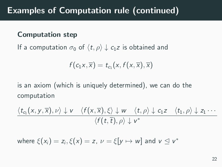
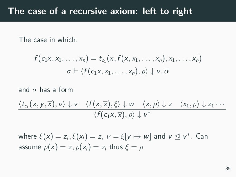
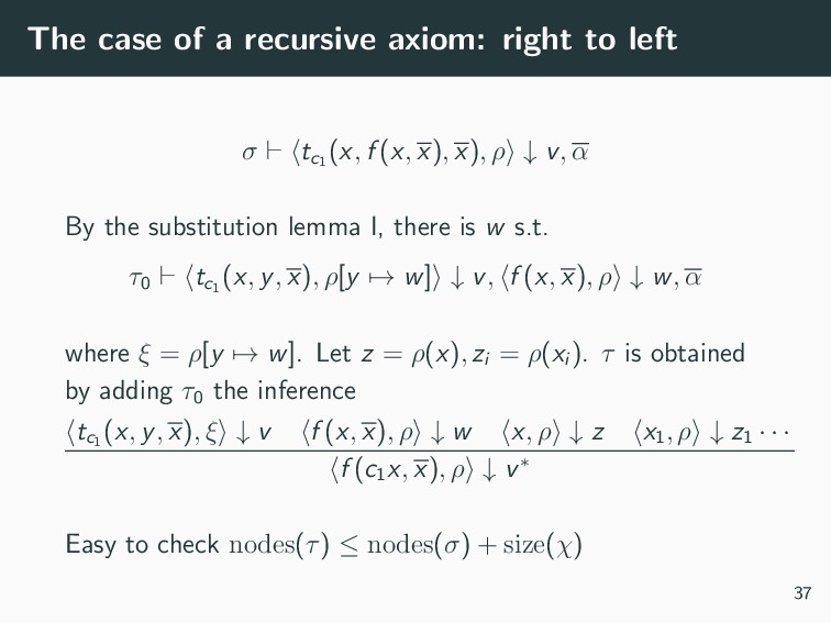
40. The case of a recursive axiom: left to right The case in which: f (c1 x, x1 , . . . , xn ) = tc1 (x, f (x, x1 , . . . , xn ), x1 , . . . , xn ) σ f (c1 x, x1 , . . . , xn ), ρ ↓ v, α and σ has a form tc1 (x, y, x), ν ↓ v f (x, x), ξ ↓ w x, ρ ↓ z x1 , ρ ↓ z1 · · · f (c1 x, x), ρ ↓ v∗ where ξ(x) = zi , ξ(xi ) = z, ν = ξ[y → w] and v v∗. Can assume ρ(x) = z, ρ(xi ) = zi thus ξ = ρ 35
41. The case of a recursive axiom: left to right (contin- ued) Make tc1 (x, y, x), ν ↓ v a conclusion. Since ν = ξ[y → w] and f (x, x), ξ ↓ w is contained in σ, apply the substitution lemma II. τ0 tc1 (x, f (x, x), x), ρ ↓ v, α Can replace ν to ρ because y disappears τ tc1 (x, f (x, x), x), ρ ↓ v, α nodes(τ) ≤ nodes(σ) + size(tc1 (#, #, #)) ≤ nodes(σ) + size(χ) 36
42. The case of a recursive axiom: right to left σ tc1 (x, f (x, x), x), ρ ↓ v, α By the substitution lemma I, there is w s.t. τ0 tc1 (x, y, x), ρ[y → w] ↓ v, f (x, x), ρ ↓ w, α where ξ = ρ[y → w]. Let z = ρ(x), zi = ρ(xi ). τ is obtained by adding τ0 the inference tc1 (x, y, x), ξ ↓ v f (x, x), ρ ↓ w x, ρ ↓ z x1 , ρ ↓ z1 · · · f (c1 x, x), ρ ↓ v∗ Easy to check nodes(τ) ≤ nodes(σ) + size(χ) 37
43. The case of the substitution rule . . . . χ0 t(x) = u(x) t(r) = u(r) Construct a computation τ u(r), ρ ↓ v, α from σ t(r), ρ ↓ v, α 38
44. The case of the substitution rule (continued) By the substitution lemma I, there is a w s.t. σ0 t(x), ρ[x → w] ↓ v, r, ρ ↓ w, α Claim σ0 satisfies the assumptions of induction hypothesis Proof. Condition 1 is trivial. Condition 2: nodes(w) ≤ max(B(α), B(ρ), T(t(r), α)) + nodes(σ) ≤ max((U − size(χ))2, size(χ)) + U − size(χ) ≤ (U − size(χ))2 + U − size(χ) ≤ (U − size(χ0 ))2 ∴ B(ρ[x → w]) ≤ (U − size(χ0 ))2 39
45. The case of the substitution rule (continued) Condition 3: M( r, ρ ↓ w, α) ≤ max(size(χ), U − size(χ)) ≤ U − size(χ) ≤ U − size(χ0 ) Condition 4: nodes(σ0 ) ≤ nodes(σ) + size(t(#)) + 1 ≤ U − size(χ) + size(t(#)) + 1 ≤ U − size(χ0 ) The claim is proved 40
46. The case of the substitution rule (continued) Therefore, apply induction hypothesis to σ0 and obtain τ0 u(x), ρ[x → w] ↓ v, r, ρ ↓ w, α By the substitution lemma II, τ u(r), ρ ↓ v, α nodes(τ) ≤ nodes(σ) + size(t(#)) + 1+ size(χ0 ) + 1 + size(u(#)) ≤ nodes(σ) + size(χ) 41
47. References i Beckmann, A. (2002). Proving consistency of equational theories in bounded arithmetic. Journal of Symbolic Logic, 67(1):279–296. Buss, S. R. and Ignjatovi´ c, A. (1995). Unprovability of consistency statements in fragments of bounded arithmetic. Annals of pure and applied Logic, 74:221–244. 42
48. References ii Yamagata, Y. (2018). Consistency proof of a fragment of pv with substitution in bounded arithmetic. The Journal of Symbolic Logic, 83(3):1063–1090. 43