Individual-based epidemiological model of COVID19 using location data

Transcript

1. Individual-based epidemiological model of COVID19 using location data Yoriyuki Yamagata*, Shunsuke Takami*, Keisuke Yamazaki*, Tomoki Nakaya**, Masaki Onishi* 2022/12/17 BDA4HM *National Institute of Advanced Industrial Science and Technology (AIST) **Tohoku University
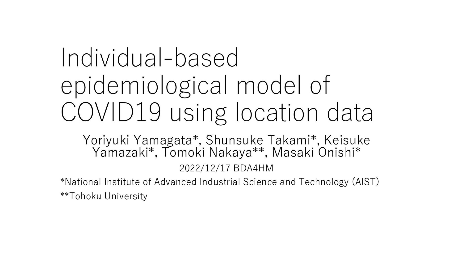
2. Context We restrict our study to year 2020, to avoid the complication of new variants and vaccination • Japan experienced the first wave around Apr. 2020 • The government asked voluntary mobility restriction during this period • This period corresponds large drop of mobility • Tokyo also experienced 2nd and 3rd waves in Aug. and Dec. 1st wave 2nd wave 3rd wave New cases and mobility in Tokyo Cases: the number of cases by infection dates, Mobility: Googleʼs community mobility report, transit stations
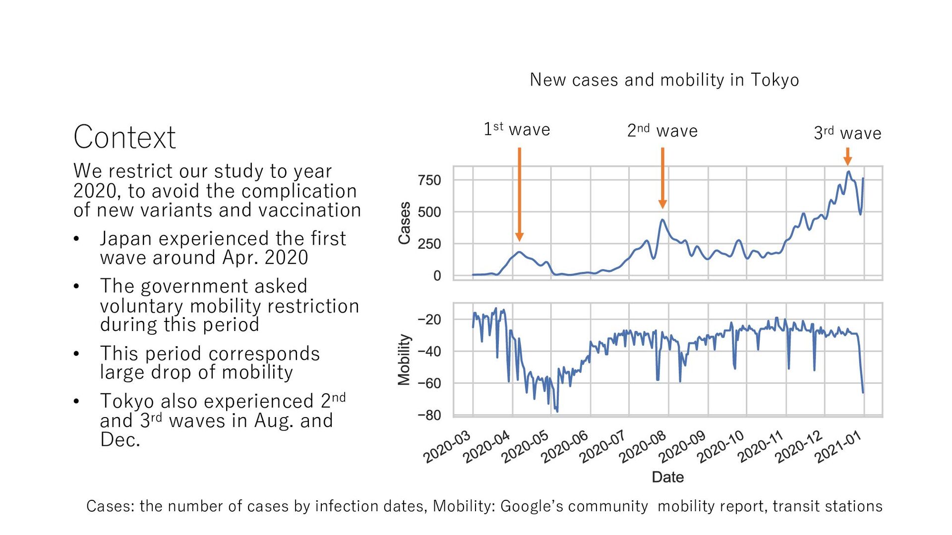
3. Motivation Mobility restriction was used by many government during COVID19 pandemic However, the decoupling of the mobility and infection was observed internationally after the initial stage of the pandemic (Gatalo 2021, Nouvellet 2021) In Tokyo, no significant correlation was observed between the effective reproduction number (Rt) and mobility after July. 2020 Rt Mobility Cor. = 0.172, p=0.400 Mobility: Googleʼs community mobility report, transit stations Effective Reproduction number (Rt) and mobility in Tokyo after July 2020
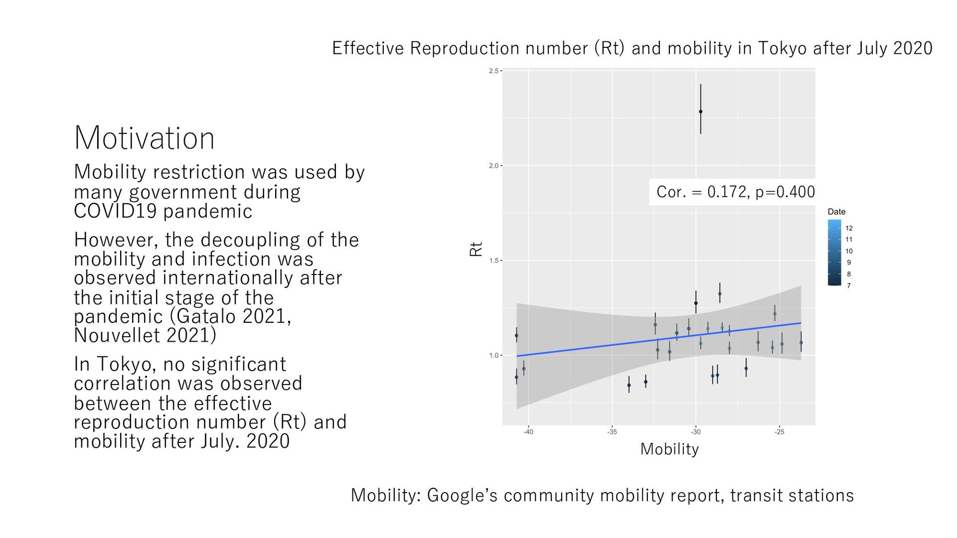
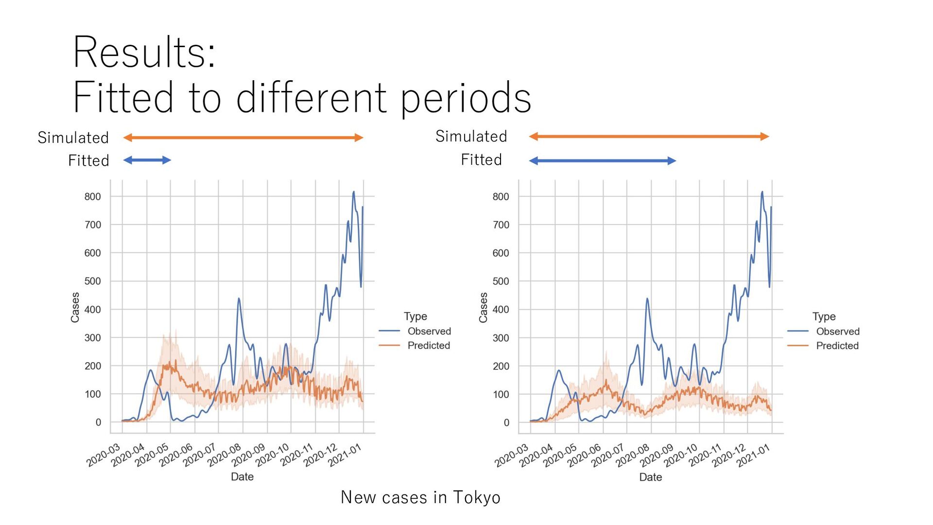
4. Contribution 1. A stochastic epidemiological model based on the movement of individuals 2. Applied the model to 10 months study period 2020-03- 01~2020-12-31, to the nation- wide 500,000 people 3. Successfully reproduced the occurrence of three waves of epidemic by fine-scale mobility, though with large difference from observed values May suggest the fine-scale mobility still affected the later stage of epidemic Tokyoʼs num of cases, observed and simulated Simulated Orange line: average, band: standard deviation of 120 runs Simulation was nation-wide but only Tokyoʼs cases are presented Jitter of simulated values caused by the weekday effect, while observed values are 7 days rolled average
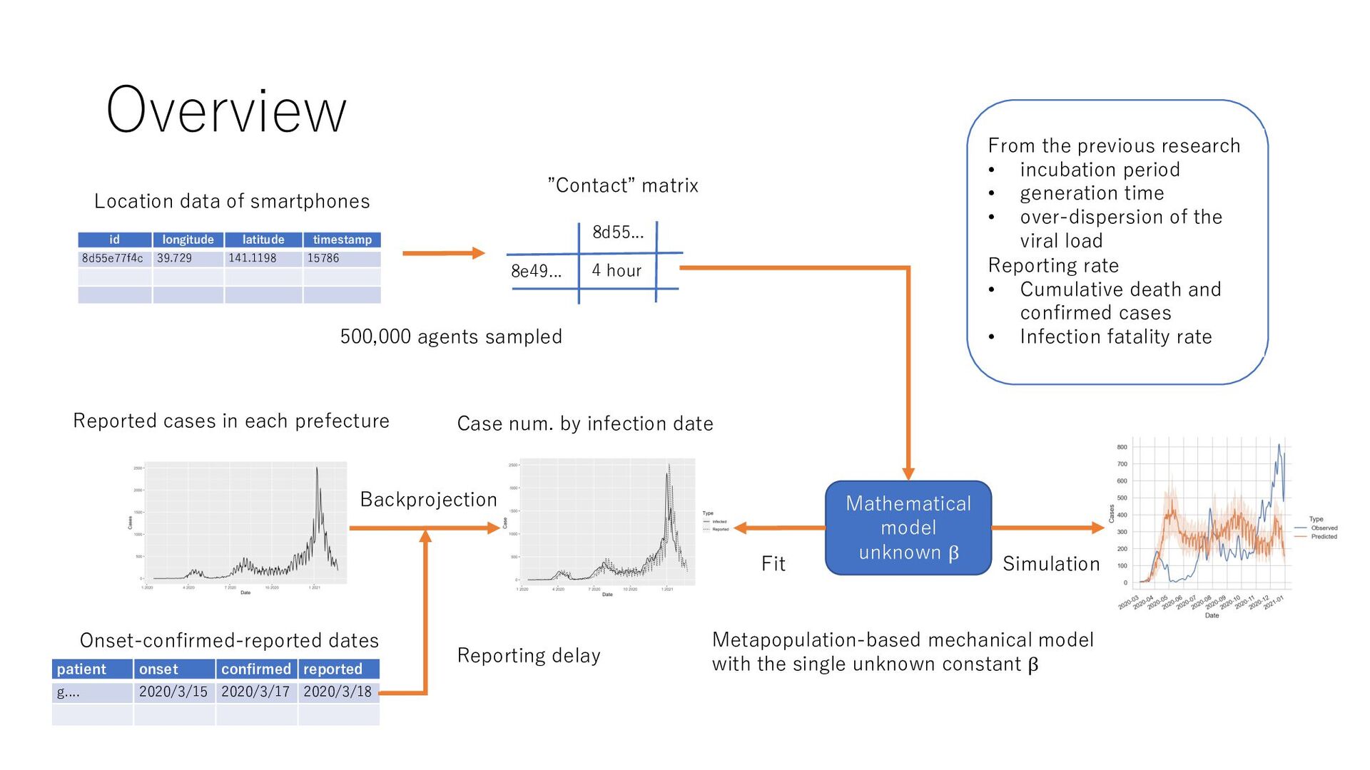
5. Overview id longitude latitude timestamp 8d55e77f4c 39.729 141.1198 15786 Location data of smartphones patient onset confirmed reported g.... 2020/3/15 2020/3/17 2020/3/18 Reported cases in each prefecture Onset-confirmed-reported dates Case num. by infection date Reporting delay Backprojection 4 hour 8d55... 8e49... ”Contact” matrix 500,000 agents sampled Mathematical model unknown β Fit Simulation Metapopulation-based mechanical model with the single unknown constant β From the previous research • incubation period • generation time • over-dispersion of the viral load Reporting rate • Cumulative death and confirmed cases • Infection fatality rate
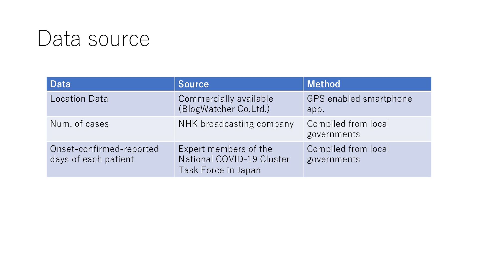
6. Data source Data Source Method Location Data Commercially available (BlogWatcher Co.Ltd.) GPS enabled smartphone app. Num. of cases NHK broadcasting company Compiled from local governments Onset-confirmed-reported days of each patient Expert members of the National COVID-19 Cluster Task Force in Japan Compiled from local governments
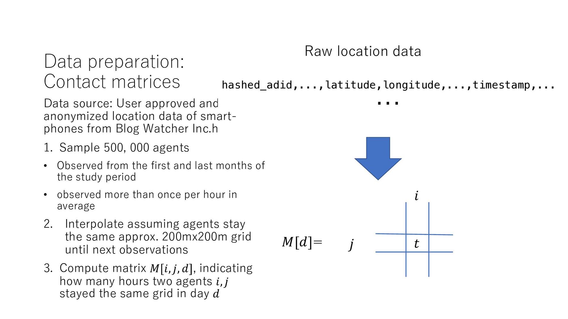
7. Data preparation: Contact matrices Data source: User approved and anonymized location data of smart- phones from Blog Watcher Inc.h 1. Sample 500, 000 agents • Observed from the first and last months of the study period • observed more than once per hour in average 2. Interpolate assuming agents stay the same approx. 200mx200m grid until next observations 3. Compute matrix 𝑀[𝑖, 𝑗, 𝑑], indicating how many hours two agents 𝑖, 𝑗 stayed the same grid in day 𝑑 hashed_adid,...,latitude,longitude,...,timestamp,... ... Raw location data 𝑖 𝑗 𝑡 𝑀[𝑑]=
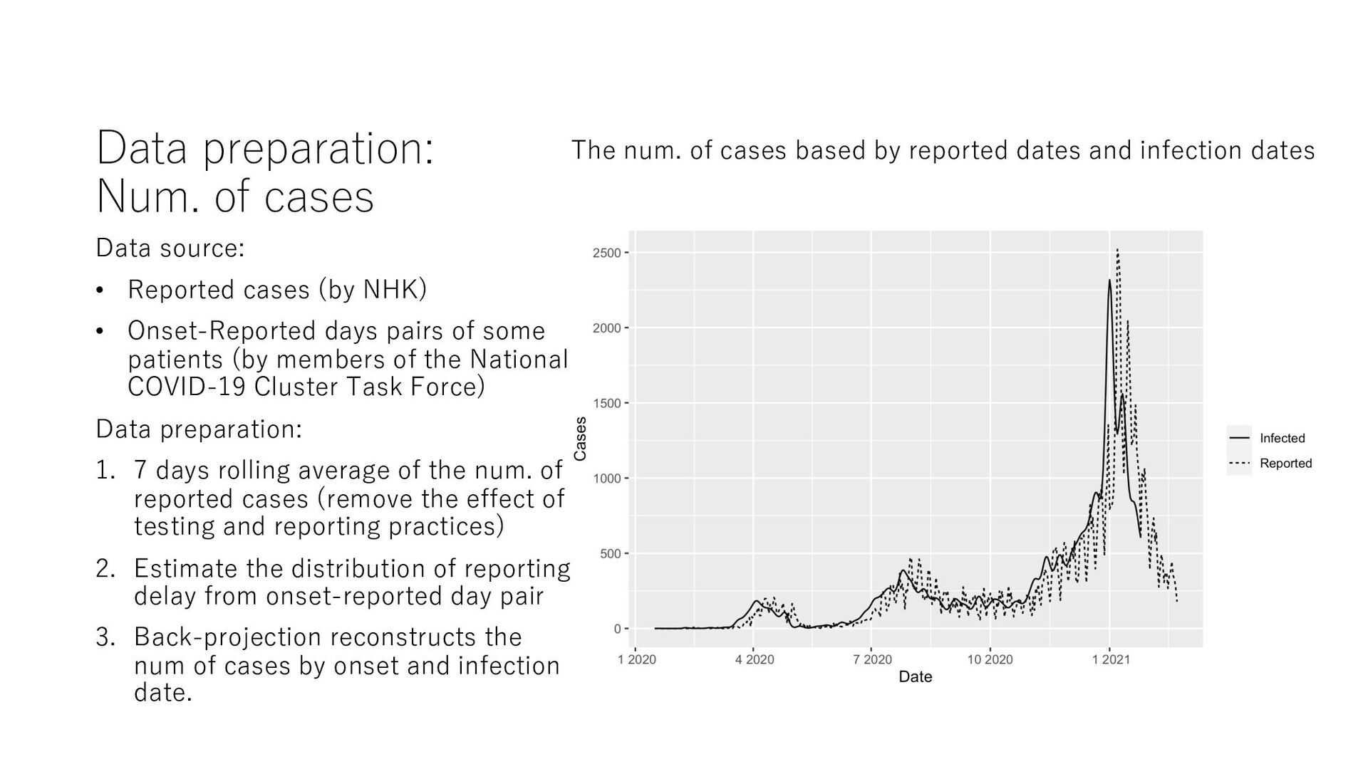
8. Data preparation: Num. of cases Data source: • Reported cases (by NHK) • Onset-Reported days pairs of some patients (by members of the National COVID-19 Cluster Task Force) Data preparation: 1. 7 days rolling average of the num. of reported cases (remove the effect of testing and reporting practices) 2. Estimate the distribution of reporting delay from onset-reported day pair 3. Back-projection reconstructs the num of cases by onset and infection date. The num. of cases based by reported dates and infection dates
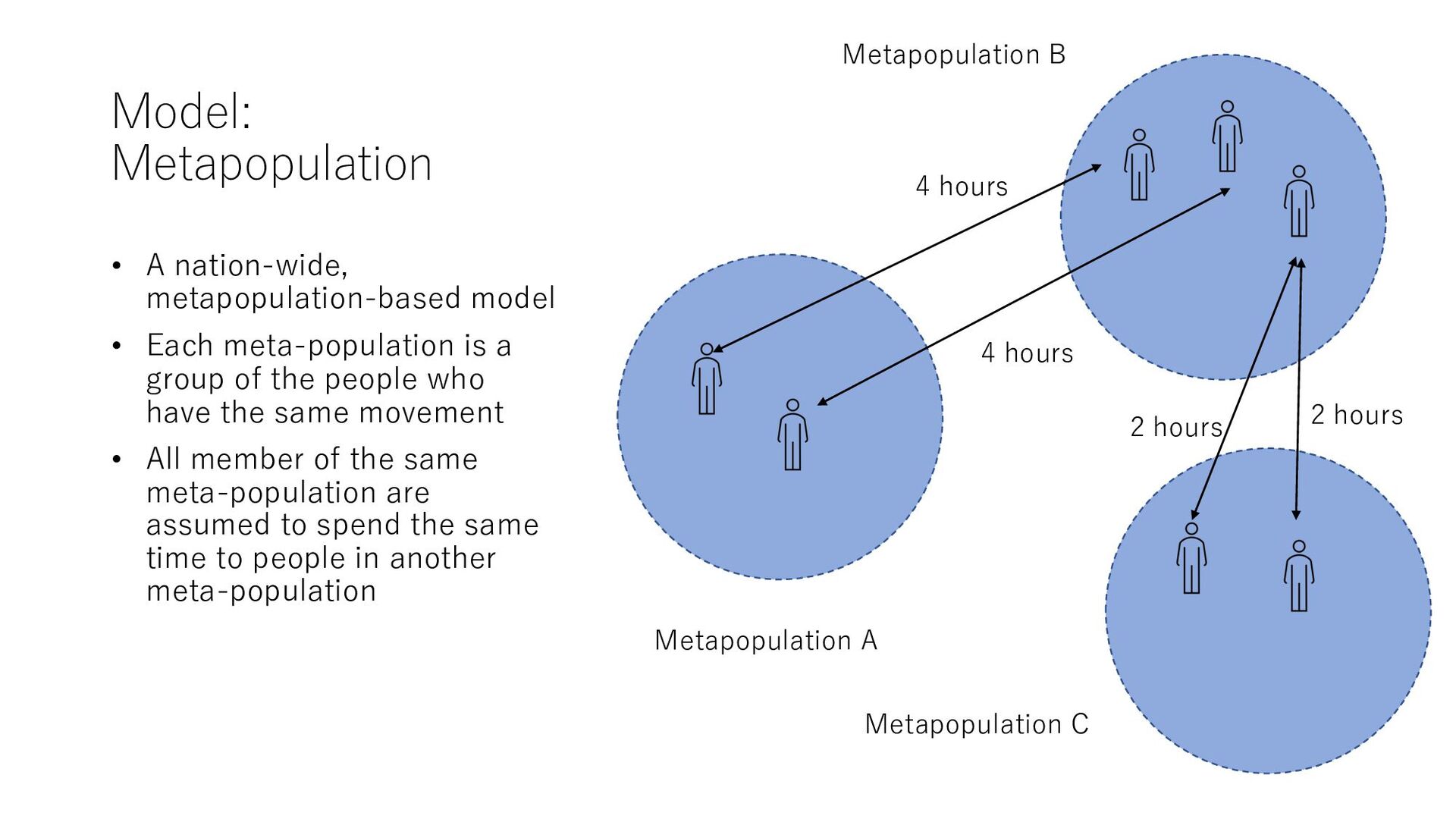
9. Model: Metapopulation • A nation-wide, metapopulation-based model • Each meta-population is a group of the people who have the same movement • All member of the same meta-population are assumed to spend the same time to people in another meta-population 4 hours 4 hours 2 hours 2 hours Metapopulation A Metapopulation B Metapopulation C
10. Model: Stochastic epidemiological model 𝑳 𝑑 ~Γ(𝐷, 𝐷/𝑰 𝑑 ) Viral load of new infected peoples 𝑬 𝑑 = 3 !"# $ 𝑔 𝑘 𝑳[𝑑 − 𝑘] Virus emission 𝑭 𝑑 = 𝑴 𝑑 𝑬[𝑑] Exposure to virus 𝑰 𝑑 + 1 ~ Binomial(𝑆 − 𝑪 𝑑 , 1 − 𝑒%&𝑭 ( ) New infection 𝑪 𝑑 + 1 = 𝑪 𝑑 + 𝑰[𝑑 + 1] Cumulative infection β: infection rate, single unknown model parameter Given: 𝑴 𝑖, 𝑗, 𝑑 : contact matrix, 𝐷:overdispersion of viral load, 𝑔 𝑘 : dist. of generation time, 𝑆: size of metapopulation
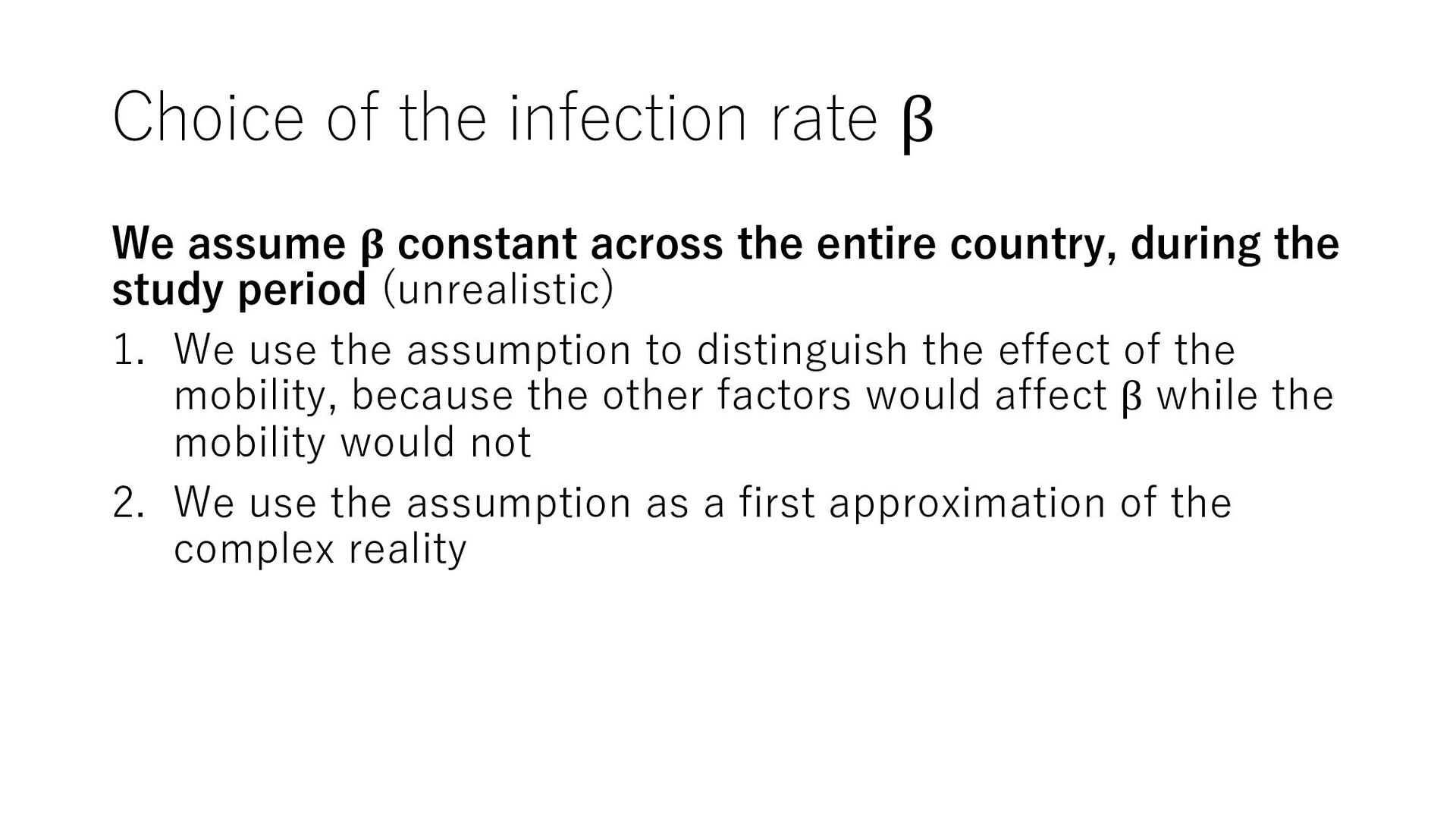
11. Choice of the infection rate β We assume 𝛃 constant across the entire country, during the study period (unrealistic) 1. We use the assumption to distinguish the effect of the mobility, because the other factors would affect β while the mobility would not 2. We use the assumption as a first approximation of the complex reality
12. Optimization Loss = ' -,. log 𝑃(𝑰. /01[𝑑] |NB(1 + ' 234 5 𝑰. 167 𝑘, 𝑑 , 1 1 + 𝑁 )) 𝑰. 167 𝑘, 𝑑 ~Binomial( ' 8 96:;1 . 𝑰167 𝑘, 𝑖, 𝑑 , 𝑞) 𝑝: a prefecture, 𝑰. /01[𝑑]: observed new infection at a prefecture 𝑝, 𝑁: num. of simulation (=30), 𝑞: reporting rate (assumed =0.5) 𝑰167 𝑘, 𝑖, 𝑑 : simulated new infection in metapopulation 𝑖, day 𝑑, simulation 𝑘 Bayesian optimization is used to find optimal β
13. Simulation • Our model has a history effect; therefore, we cannot start the simulation from an arbitrary point • We always start from Mar 1, when we can assume that the cases were evenly distributed • We ran 120 simulations and took the average and standard deviation as a prediction
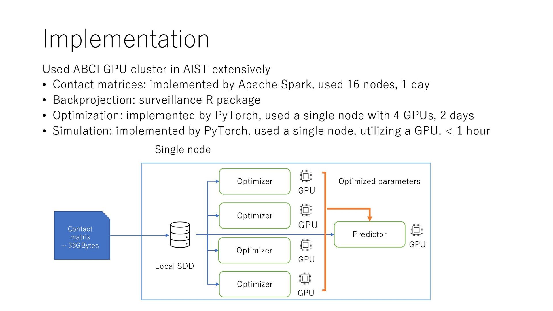
14. Implementation Used ABCI GPU cluster in AIST extensively • Contact matrices: implemented by Apache Spark, used 16 nodes, 1 day • Backprojection: surveillance R package • Optimization: implemented by PyTorch, used a single node with 4 GPUs, 2 days • Simulation: implemented by PyTorch, used a single node, utilizing a GPU, < 1 hour Contact matrix ~ 36GBytes Local SDD Predictor GPU Optimizer GPU Optimizer GPU Optimizer GPU Optimizer GPU Optimized parameters Single node
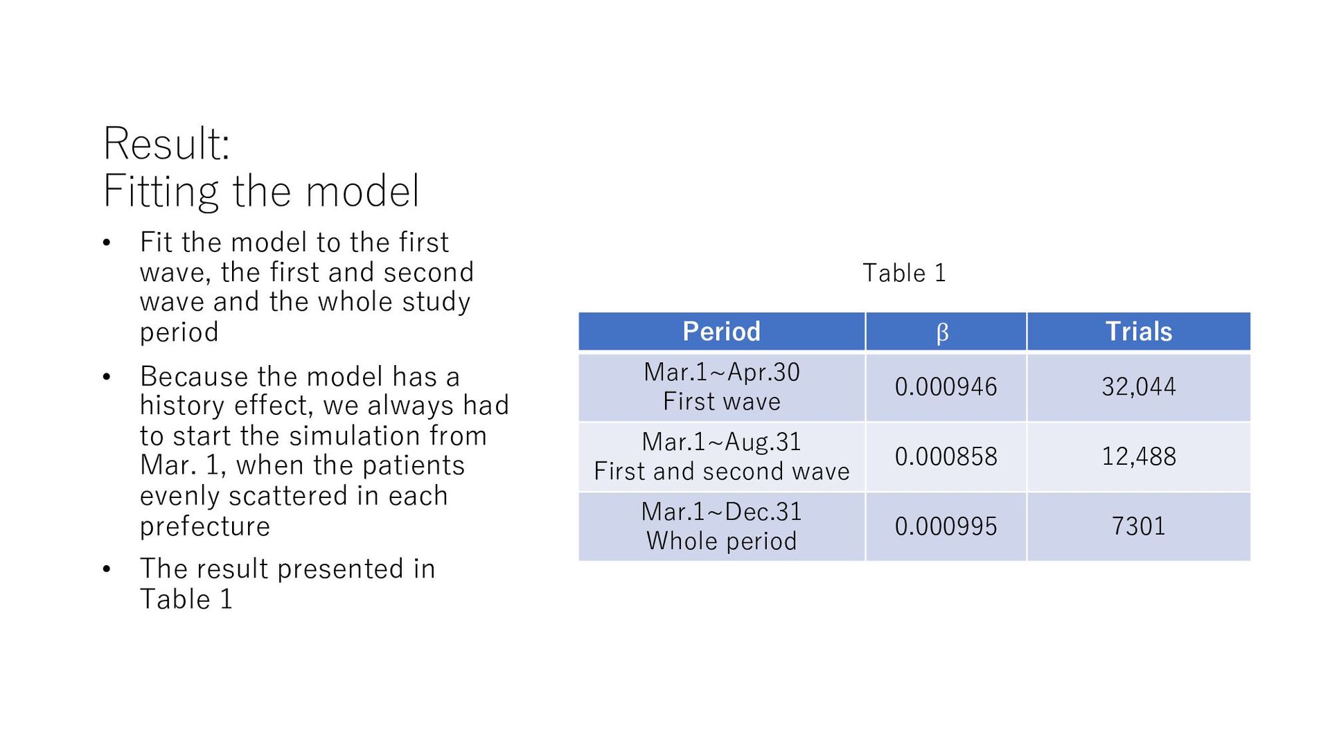
15. Result: Fitting the model Period β Trials Mar.1~Apr.30 First wave 0.000946 32,044 Mar.1~Aug.31 First and second wave 0.000858 12,488 Mar.1~Dec.31 Whole period 0.000995 7301 • Fit the model to the first wave, the first and second wave and the whole study period • Because the model has a history effect, we always had to start the simulation from Mar. 1, when the patients evenly scattered in each prefecture • The result presented in Table 1 Table 1
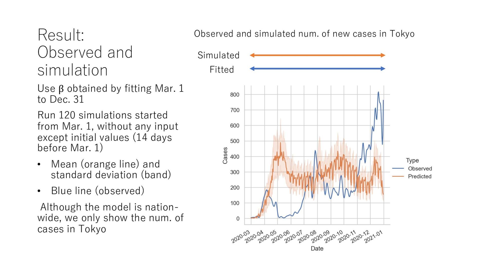
16. Result: Observed and simulation Use β obtained by fitting Mar. 1 to Dec. 31 Run 120 simulations started from Mar. 1, without any input except initial values (14 days before Mar. 1) • Mean (orange line) and standard deviation (band) • Blue line (observed) Although the model is nation- wide, we only show the num. of cases in Tokyo Observed and simulated num. of new cases in Tokyo Fitted Simulated
17. Results: Regional difference Hokkaido Shimane Fitted Simulated Fitted Simulated
18. Results: Fitted to different periods Fitted Simulated Simulated Fitted New cases in Tokyo
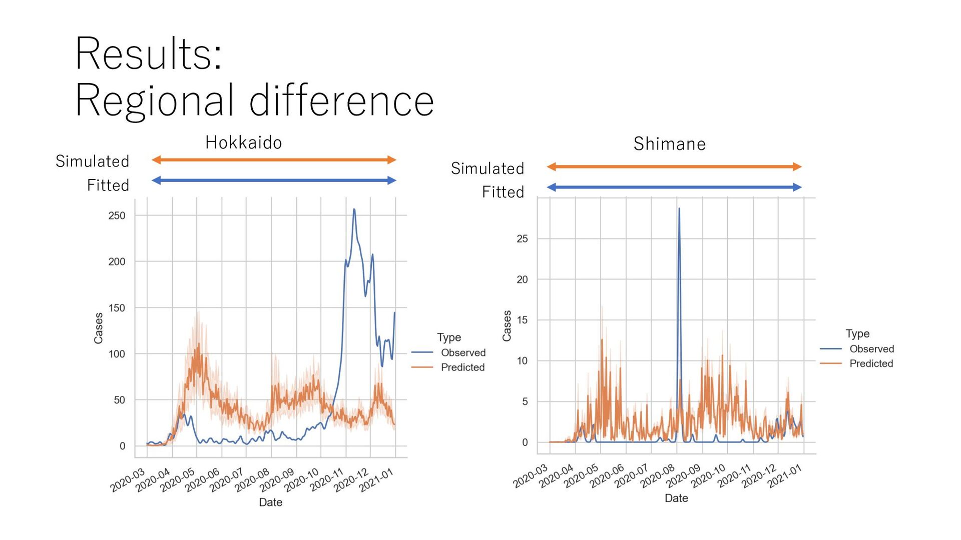
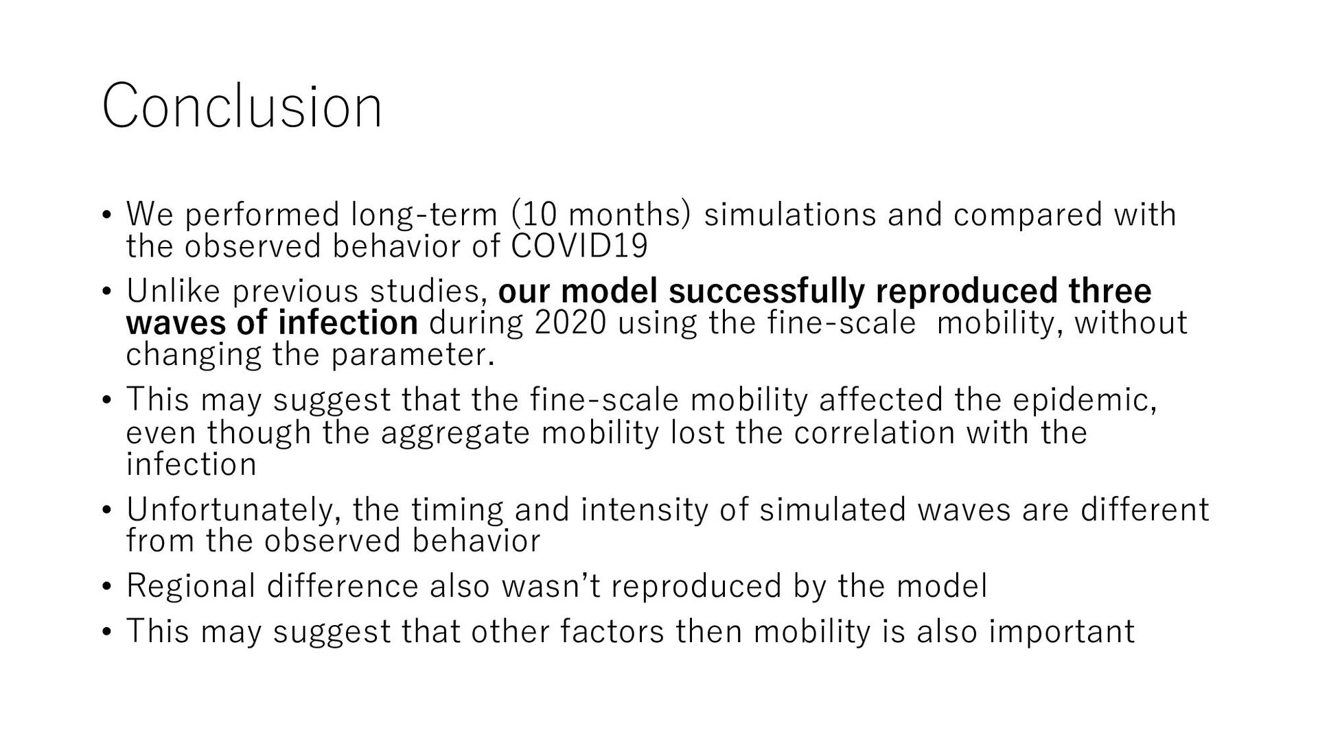
19. Conclusion • We performed long-term (10 months) simulations and compared with the observed behavior of COVID19 • Unlike previous studies, our model successfully reproduced three waves of infection during 2020 using the fine-scale mobility, without changing the parameter. • This may suggest that the fine-scale mobility affected the epidemic, even though the aggregate mobility lost the correlation with the infection • Unfortunately, the timing and intensity of simulated waves are different from the observed behavior • Regional difference also wasnʼt reproduced by the model • This may suggest that other factors then mobility is also important
20. Future work • Improve the model • Heterogeneity inside a metapopulation • Differentiate β by land usage • Multi-tier model (family, workplace, public places...) • Change β over time and regions, based on a statical model • Analyze the mechanism of the resurgence in the model • Simulate the geological pattern of infection • Incorporate new variants and vaccination • Combine with a human mobility model • Multi-agent model or machine-learning model?