CIDUE 2013

Slides describing a recent publication in the IEEE Symposium on Computational Intelligence in Dynamic and Uncertain Environments.

Transcript

1. Discounted Expert Weighting for Concept Drift Gregory Ditzler1, Robi Polikar2, and Gail Rosen1 1Drexel University, Dept. of Electrical & Computer Engineering, Philadelphia, PA, USA 2Rowan University, Dept. of Electrical & Computer Engineering, Glassboro, NJ, USA gregory.ditzler@gmail.com, polikar@rowan.edu, gailr@ece.drexel.edu April 17, 2013 Ditzler, Polikar & Rosen (Drexel/Rowan University) CIDUE (2013), Singapore April 17, 2013 1 / 15
2. Overview 1 Overview of concept drift with multiple experts 2 Experts’ weights, loss functions, and an upper bound on loss 3 Simulations & real-world data sets 4 Conclusions & discussion Dow Jones Industrial Average index with the 30 companies associated with the index 1993 1998 2004 2009 0 50 100 150 200 250 Ditzler, Polikar & Rosen (Drexel/Rowan University) CIDUE (2013), Singapore April 17, 2013 2 / 15
3. Concept Drift, Time Series, Transfer Learning and Model Adaption Time Series (time-dependent) Knowledge transfer / Transfer learning Model Adaptation Concept Drift Adapted from: I. Žliobait˙ e, “Learning under concept drift: an overview,” http://arxiv.org/abs/1010.4784, 2010. Ditzler, Polikar & Rosen (Drexel/Rowan University) CIDUE (2013), Singapore April 17, 2013 3 / 15
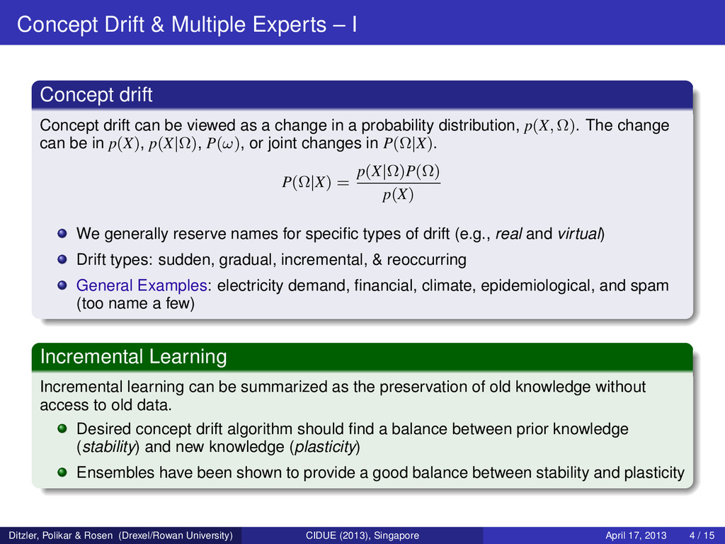
4. Concept Drift & Multiple Experts – I Concept drift Concept drift can be viewed as a change in a probability distribution, p(X, Ω). The change can be in p(X), p(X|Ω), P(ω), or joint changes in P(Ω|X). P(Ω|X) = p(X|Ω)P(Ω) p(X) We generally reserve names for specific types of drift (e.g., real and virtual) Drift types: sudden, gradual, incremental, & reoccurring General Examples: electricity demand, financial, climate, epidemiological, and spam (too name a few) Incremental Learning Incremental learning can be summarized as the preservation of old knowledge without access to old data. Desired concept drift algorithm should find a balance between prior knowledge (stability) and new knowledge (plasticity) Ensembles have been shown to provide a good balance between stability and plasticity Ditzler, Polikar & Rosen (Drexel/Rowan University) CIDUE (2013), Singapore April 17, 2013 4 / 15
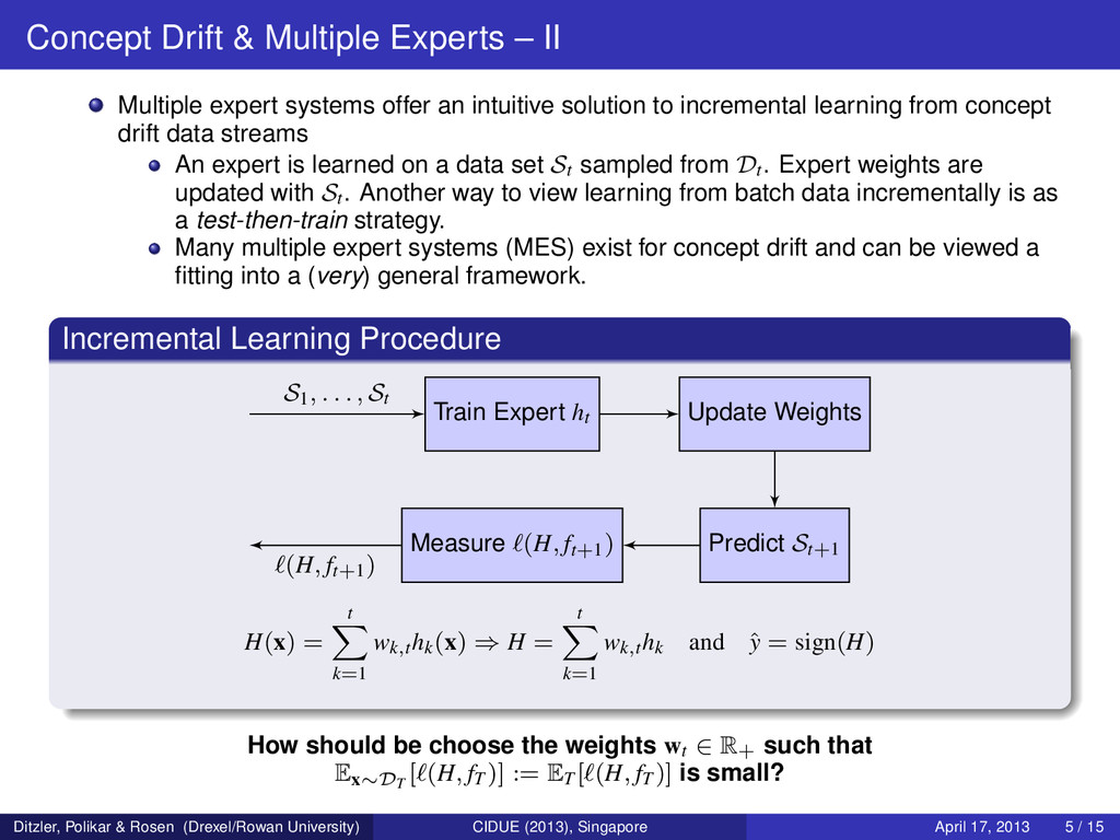
5. Concept Drift & Multiple Experts – II Multiple expert systems offer an intuitive solution to incremental learning from concept drift data streams An expert is learned on a data set St sampled from Dt. Expert weights are updated with St. Another way to view learning from batch data incrementally is as a test-then-train strategy. Many multiple expert systems (MES) exist for concept drift and can be viewed a fitting into a (very) general framework. Incremental Learning Procedure Train Expert ht Update Weights Predict St+1 Measure (H, ft+1) S1, . . . , St (H, ft+1) H(x) = t k=1 wk,thk(x) ⇒ H = t k=1 wk,thk and ˆ y = sign(H) How should be choose the weights wt ∈ R+ such that Ex∼DT [ (H, fT )] := ET [ (H, fT )] is small? Ditzler, Polikar & Rosen (Drexel/Rowan University) CIDUE (2013), Singapore April 17, 2013 5 / 15
6. Weighting Experts – I Uniform Weights & Follow-the-Leader There are several ways that the weights, wk,t, for an MES can be selected. Ideally, the selection of the weight produces a low generalization loss on future unlabeled data. DT does not come with labeled information at the time of testing; however, we have observed labels for Dt Uniform: Some have suggested that setting the weights to 1 t is optimal; however, the learning assumptions to prove this are harsh. Follow-the-Leader (FTL) may work well, but what if the divergence between DT and Dt is not negligible? Exponential Weighting The exponential weighted forecaster has be widely used by many MES, which is given by wk,t = wk,t−1 exp(−ηEt[ (hk, ft)]) t j=1 wj,t−1 exp(−ηEt[ (hj, ft)]) where η is the smoothing parameter. What if not all losses should be equally weighted? Ditzler, Polikar & Rosen (Drexel/Rowan University) CIDUE (2013), Singapore April 17, 2013 6 / 15
7. Weighting Experts – II Adaboost Style Weighting Many MES use Adaboost’s weighting scheme, where the loss is computed with the most recent training data. wk,t = log 1 − Et[ (hk, ft)] Et[ (hk, ft)] Using Et[ (hk, ft)] may not be ideal; however, examining Et [ (hk, ft )] for t < t allows us to see how well hk has performed in recent time. How well does Adaboost’s weighting compare to exponential weighting for different values of η? 0 0.1 0.2 0.3 0.4 0.5 0 0.05 0.1 0.15 0.2 0.25 0.3 0.35 E[L(h,y)] Weight Exp(5) Exp(10) Exp(20) NSE 0 0.1 0.2 0.3 0.4 0.5 0 0.05 0.1 0.15 0.2 E[L(h,y)] Weight Exp(5) Exp(10) Exp(20) NSE Ditzler, Polikar & Rosen (Drexel/Rowan University) CIDUE (2013), Singapore April 17, 2013 7 / 15
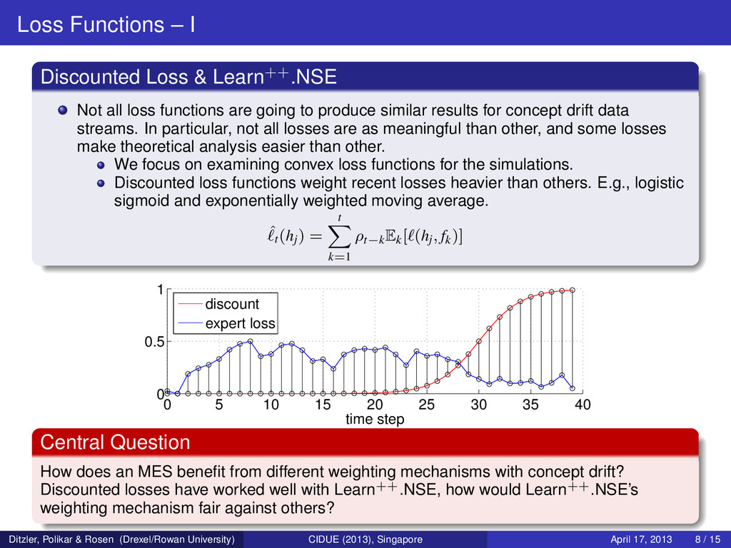
8. Loss Functions – I Discounted Loss & Learn++.NSE Not all loss functions are going to produce similar results for concept drift data streams. In particular, not all losses are as meaningful than other, and some losses make theoretical analysis easier than other. We focus on examining convex loss functions for the simulations. Discounted loss functions weight recent losses heavier than others. E.g., logistic sigmoid and exponentially weighted moving average. ˆ t(hj) = t k=1 ρt−kEk[ (hj, fk)] 0 5 10 15 20 25 30 35 40 0 0.5 1 time step discount expert loss Central Question How does an MES benefit from different weighting mechanisms with concept drift? Discounted losses have worked well with Learn++.NSE, how would Learn++.NSE’s weighting mechanism fair against others? Ditzler, Polikar & Rosen (Drexel/Rowan University) CIDUE (2013), Singapore April 17, 2013 8 / 15
9. Upper Bound on Loss What is the loss on DT for an MES? Assuming that is convex in the first argument then by linearity of expectation and Jenson’s inequality, we have ET [ (H, fT )] ≤ t k=1 wk,tET [ (hk, fT )] where fT is the true labeling function of the target. Post-CIDUE work has developed a more concrete bound using recent mathematical tools from domain adaptation. Generally not computable since we do not have access to fT Central Question Given the general bound shown above, which typically cannot be computed, what weighting scheme can provide the tightest upper bound when the loss is viewed as a stochastic process? Loss is a Markov process and fits the properties of concept drift as described by Gao et al. (2009) Ditzler, Polikar & Rosen (Drexel/Rowan University) CIDUE (2013), Singapore April 17, 2013 9 / 15
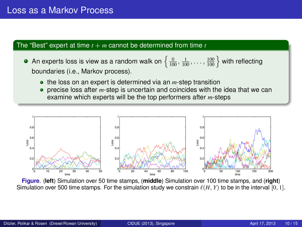
10. Loss as a Markov Process The “Best” expert at time t + m cannot be determined from time t An experts loss is view as a random walk on 0 100 , 1 100 , . . . , 100 100 with reflecting boundaries (i.e., Markov process). the loss on an expert is determined via an m-step transition precise loss after m-step is uncertain and coincides with the idea that we can examine which experts will be the top performers after m-steps 0 10 20 30 40 50 0 0.2 0.4 0.6 0.8 1 time Loss 0 20 40 60 80 100 0 0.2 0.4 0.6 0.8 1 time Loss 0 50 100 150 200 0 0.2 0.4 0.6 0.8 1 time Loss Figure. (left) Simulation over 50 time stamps, (middle) Simulation over 100 time stamps, and (right) Simulation over 500 time stamps. For the simulation study we constrain (H, Y) to be in the interval [0, 1]. Ditzler, Polikar & Rosen (Drexel/Rowan University) CIDUE (2013), Singapore April 17, 2013 10 / 15
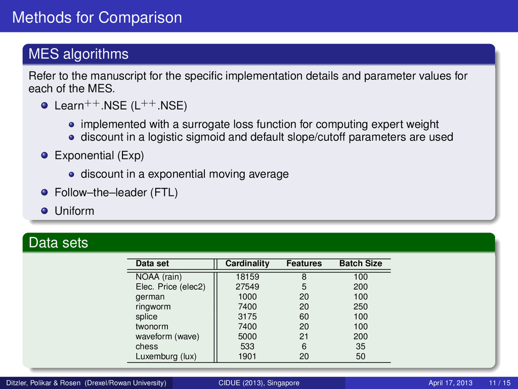
11. Methods for Comparison MES algorithms Refer to the manuscript for the specific implementation details and parameter values for each of the MES. Learn++.NSE (L++.NSE) implemented with a surrogate loss function for computing expert weight discount in a logistic sigmoid and default slope/cutoff parameters are used Exponential (Exp) discount in a exponential moving average Follow–the–leader (FTL) Uniform Data sets Data set Cardinality Features Batch Size NOAA (rain) 18159 8 100 Elec. Price (elec2) 27549 5 200 german 1000 20 100 ringworm 7400 20 250 splice 3175 60 100 twonorm 7400 20 100 waveform (wave) 5000 21 200 chess 533 6 35 Luxemburg (lux) 1901 20 50 Ditzler, Polikar & Rosen (Drexel/Rowan University) CIDUE (2013), Singapore April 17, 2013 11 / 15
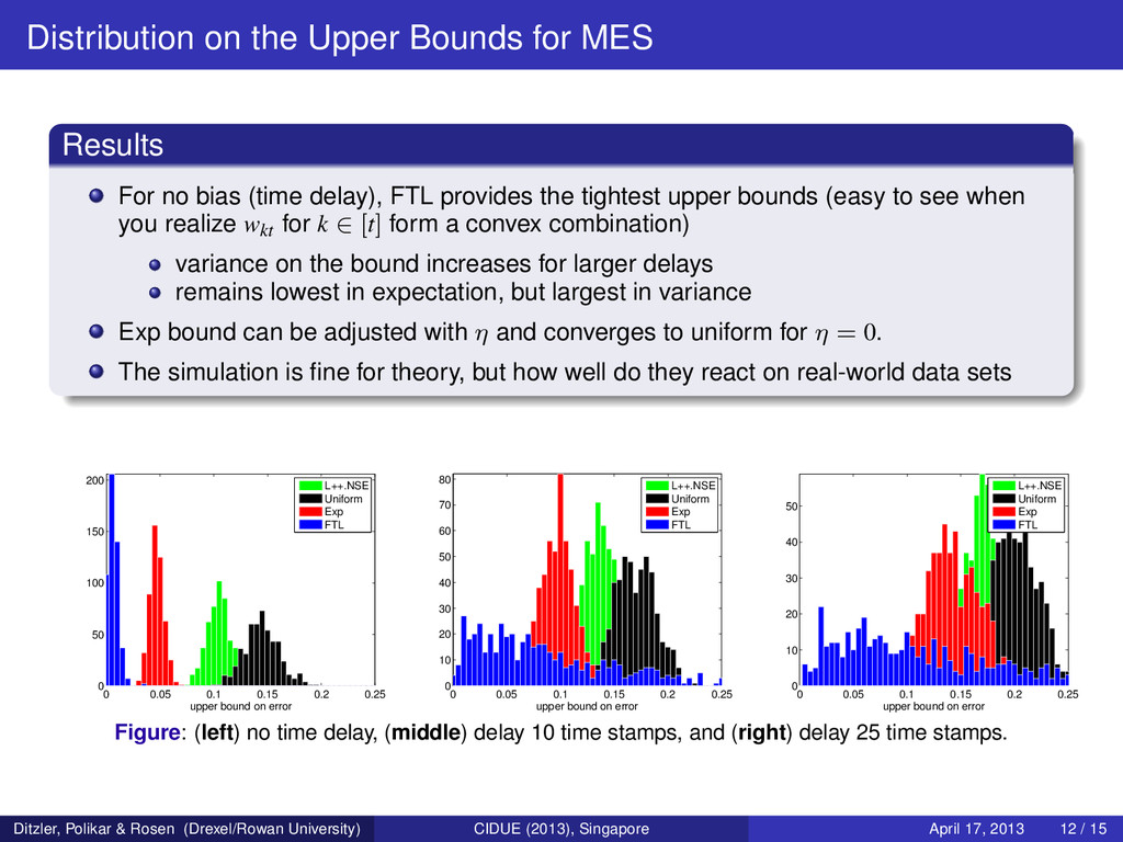
12. Distribution on the Upper Bounds for MES Results For no bias (time delay), FTL provides the tightest upper bounds (easy to see when you realize wkt for k ∈ [t] form a convex combination) variance on the bound increases for larger delays remains lowest in expectation, but largest in variance Exp bound can be adjusted with η and converges to uniform for η = 0. The simulation is fine for theory, but how well do they react on real-world data sets 0 0.05 0.1 0.15 0.2 0.25 0 50 100 150 200 upper bound on error L++.NSE Uniform Exp FTL 0 0.05 0.1 0.15 0.2 0.25 0 10 20 30 40 50 60 70 80 upper bound on error L++.NSE Uniform Exp FTL 0 0.05 0.1 0.15 0.2 0.25 0 10 20 30 40 50 upper bound on error L++.NSE Uniform Exp FTL Figure: (left) no time delay, (middle) delay 10 time stamps, and (right) delay 25 time stamps. Ditzler, Polikar & Rosen (Drexel/Rowan University) CIDUE (2013), Singapore April 17, 2013 12 / 15
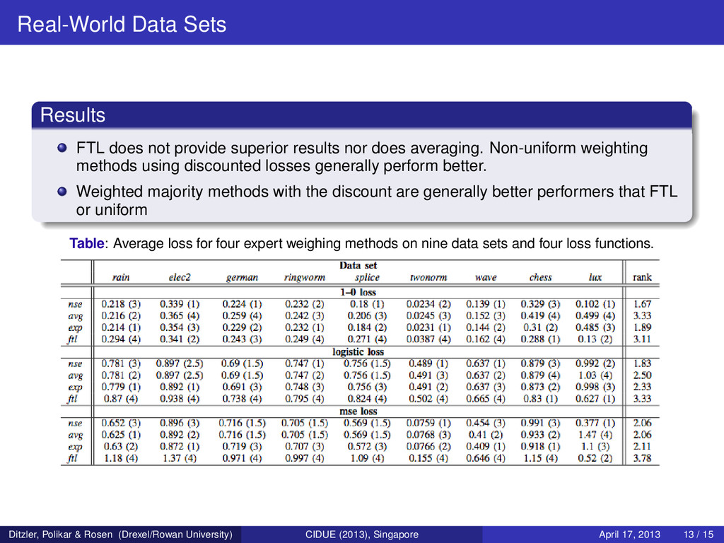
13. Real-World Data Sets Results FTL does not provide superior results nor does averaging. Non-uniform weighting methods using discounted losses generally perform better. Weighted majority methods with the discount are generally better performers that FTL or uniform Table: Average loss for four expert weighing methods on nine data sets and four loss functions. Ditzler, Polikar & Rosen (Drexel/Rowan University) CIDUE (2013), Singapore April 17, 2013 13 / 15
14. Conclusion Final Remarks Summary: We examined an upper bound on the loss on several MES by considering different weighting schemes. A stochastic loss was simulated, and the MES were tested across multiple loss functions. FTL while producing tight bounds for low bias systems becomes highly variable when the bias increases Weighted majority type MES appear to provide tighter bounds than uniform weights We tested on real-world streams discounted losses perform well in concept drift situations Future Work Develop a more definitive upper bound on the loss of the MES using recent techniques for domain adaption. Ditzler, Polikar & Rosen (Drexel/Rowan University) CIDUE (2013), Singapore April 17, 2013 14 / 15
15. Acknowledgments Funding Gregory Ditzler and Gail Rosen are supported by National Science Foundation [#0845827], [#1120622], and the Department of Energy Award [#SC004335]. Robi Polikar is supported by the National Science Foundation [ECCS-0926159]. Ditzler, Polikar & Rosen (Drexel/Rowan University) CIDUE (2013), Singapore April 17, 2013 15 / 15