Joint modelling of multivariate longitudinal and time-to-event data

Conference presentation from the 9th International Conference of the ERCIM WG on Computational and Methodological Statistics, Seville, Spain (10th December, 2016)

Transcript

1. Introduction Model Estimation Simulation Software Example Summary References Joint modelling of multivariate longitudinal and time-to-event data Graeme L. Hickey Department of Biostatistics, University of Liverpool, UK graeme.hickey@liverpool.ac.uk 9th International Conference of the ERCIM WG on Computational and Methodological Statistics, Seville, Spain GL. Hickey Joint modelling of multivariate data
2. Introduction Model Estimation Simulation Software Example Summary References Outline of talk 1 Introduction 2 Model 3 Estimation 4 Simulation 5 Software 6 Example 7 Summary GL. Hickey Joint modelling of multivariate data
3. Introduction Model Estimation Simulation Software Example Summary References Motivation for multivariate joint models Clinical studies often repeatedly measure multiple biomarkers or other measurements and an event time Research has predominantly focused on a single event time and single measurement outcome Ignoring correlation leads to bias and reduced efficiency in estimation Harnessing all available information in a single model is advantageous and should lead to improved model predictions GL. Hickey Joint modelling of multivariate data
4. Introduction Model Estimation Simulation Software Example Summary References What is the state of the field? A large number of models published over recent years incorporating different outcome types; distributions, multivariate event times; estimation approaches; association structures; disease areas; etc. Early adoption into clinical literature, but a lack of software! GL. Hickey Joint modelling of multivariate data
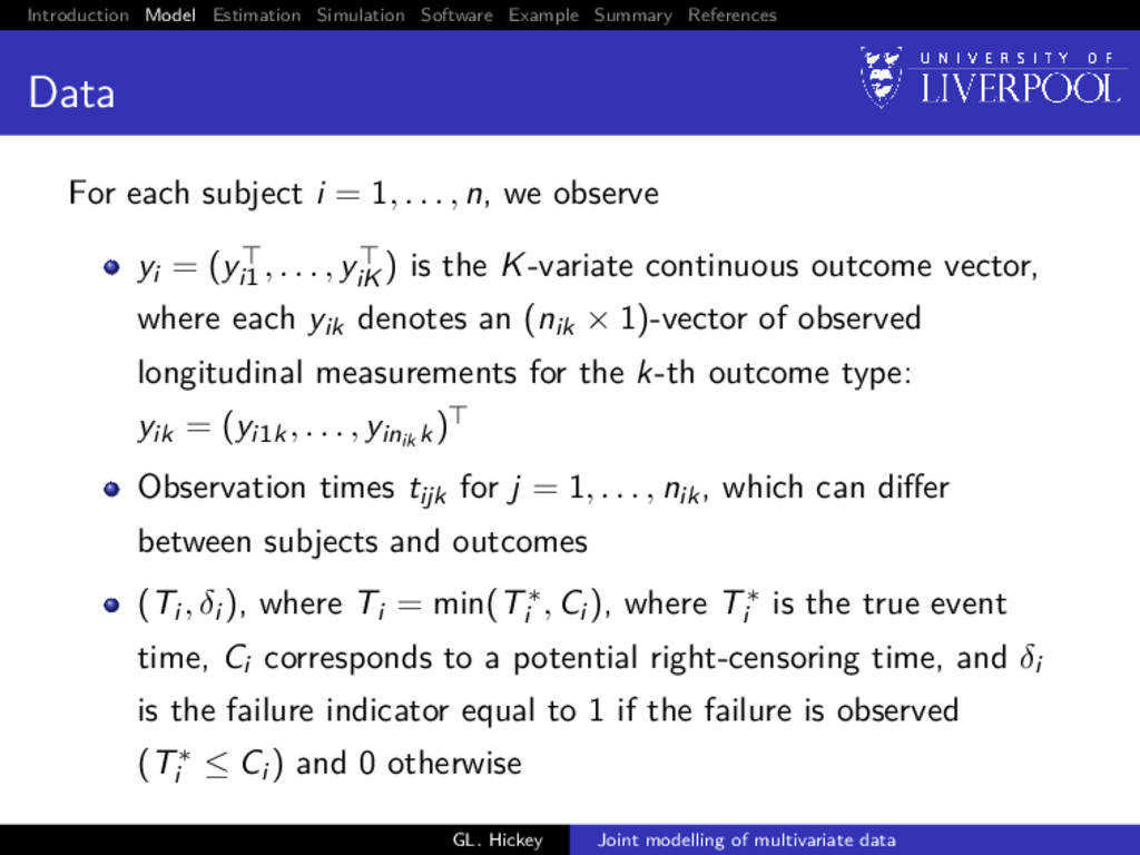
5. Introduction Model Estimation Simulation Software Example Summary References Data For each subject i = 1, . . . , n, we observe yi = (yi1 , . . . , yiK ) is the K-variate continuous outcome vector, where each yik denotes an (nik × 1)-vector of observed longitudinal measurements for the k-th outcome type: yik = (yi1k, . . . , yinik k) Observation times tijk for j = 1, . . . , nik, which can differ between subjects and outcomes (Ti , δi ), where Ti = min(T∗ i , Ci ), where T∗ i is the true event time, Ci corresponds to a potential right-censoring time, and δi is the failure indicator equal to 1 if the failure is observed (T∗ i ≤ Ci ) and 0 otherwise GL. Hickey Joint modelling of multivariate data
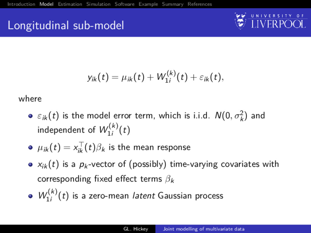
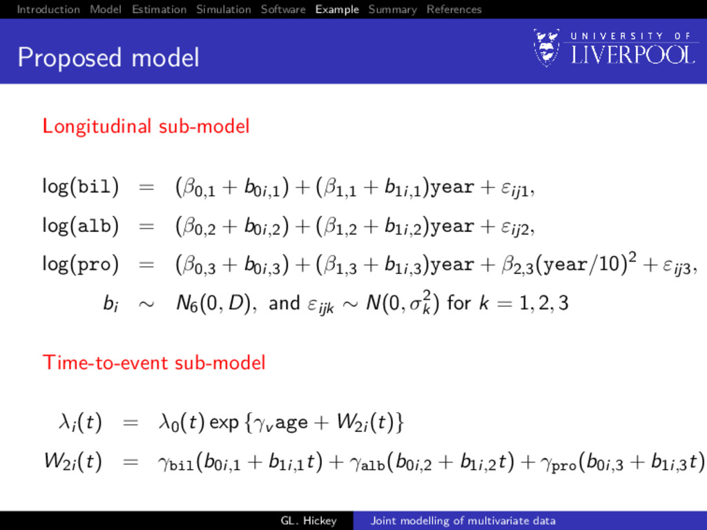
6. Introduction Model Estimation Simulation Software Example Summary References Longitudinal sub-model yik(t) = µik(t) + W (k) 1i (t) + εik(t), where εik(t) is the model error term, which is i.i.d. N(0, σ2 k ) and independent of W (k) 1i (t) µik(t) = xik (t)βk is the mean response xik(t) is a pk-vector of (possibly) time-varying covariates with corresponding fixed effect terms βk W (k) 1i (t) is a zero-mean latent Gaussian process GL. Hickey Joint modelling of multivariate data
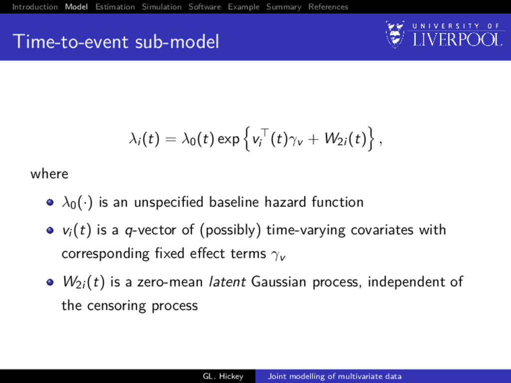
7. Introduction Model Estimation Simulation Software Example Summary References Time-to-event sub-model λi (t) = λ0(t) exp vi (t)γv + W2i (t) , where λ0(·) is an unspecified baseline hazard function vi (t) is a q-vector of (possibly) time-varying covariates with corresponding fixed effect terms γv W2i (t) is a zero-mean latent Gaussian process, independent of the censoring process GL. Hickey Joint modelling of multivariate data
8. Introduction Model Estimation Simulation Software Example Summary References Association structure Following Laird and Ware (1982): W (k) 1i (t) = zik (t)bik GL. Hickey Joint modelling of multivariate data
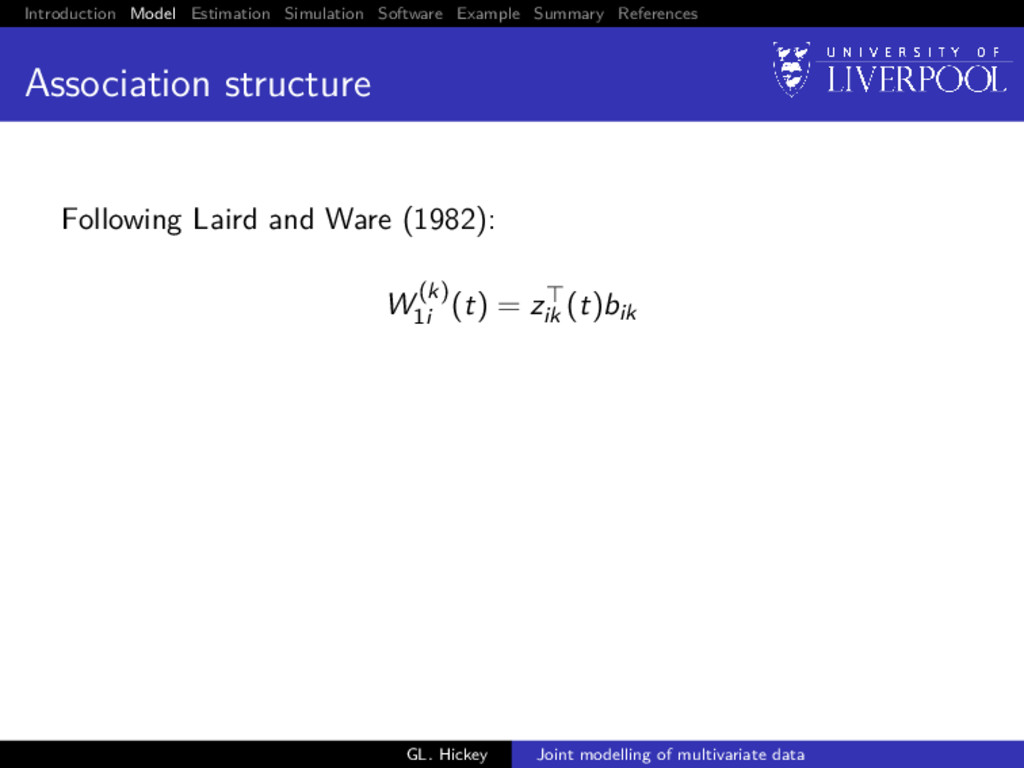
9. Introduction Model Estimation Simulation Software Example Summary References Association structure Following Laird and Ware (1982): W (k) 1i (t) = zik (t)bik 1 Within-subject correlation between longitudinal measurements: bik ∼ N(0, Dkk) GL. Hickey Joint modelling of multivariate data
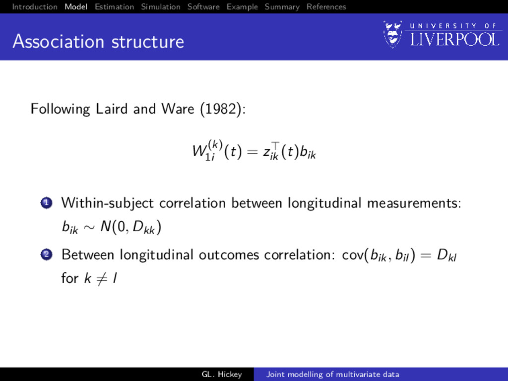
10. Introduction Model Estimation Simulation Software Example Summary References Association structure Following Laird and Ware (1982): W (k) 1i (t) = zik (t)bik 1 Within-subject correlation between longitudinal measurements: bik ∼ N(0, Dkk) 2 Between longitudinal outcomes correlation: cov(bik, bil ) = Dkl for k = l GL. Hickey Joint modelling of multivariate data
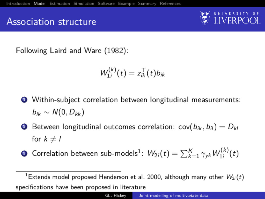
11. Introduction Model Estimation Simulation Software Example Summary References Association structure Following Laird and Ware (1982): W (k) 1i (t) = zik (t)bik 1 Within-subject correlation between longitudinal measurements: bik ∼ N(0, Dkk) 2 Between longitudinal outcomes correlation: cov(bik, bil ) = Dkl for k = l 3 Correlation between sub-models1: W2i (t) = K k=1 γykW (k) 1i (t) 1Extends model proposed Henderson et al. 2000, although many other W2i (t) specifications have been proposed in literature GL. Hickey Joint modelling of multivariate data
12. Introduction Model Estimation Simulation Software Example Summary References Estimation The estimation methodology mainly follows the 3 seminal works: 1 Wulfsohn, MS and Tsiatis, AA (1997). A joint model for survival and longitudinal data measured with error. Biometrics 53(1), pp. 330–339 2 Henderson, R et al. (2000). Joint modelling of longitudinal measurements and event time data. Biostatistics 1(4), pp. 465–480 3 Lin, H et al. (2002). Maximum likelihood estimation in the joint analysis of time-to-event and multiple longitudinal variables. Stat Med 21, pp. 2369–2382 Lin et al. (2002) is specific to multivariate longitudinal data GL. Hickey Joint modelling of multivariate data
13. Introduction Model Estimation Simulation Software Example Summary References Likelihood We can re-write the longitudinal sub-model as yi | bi , β, Σi ∼ N(Xi β + Zi bi , Σi ), with bi | D ∼ N(0, D), where β = (β1 , . . . , βK ), and Xi =      Xi1 · · · 0 . . . ... . . . 0 · · · XiK      , Zi =      Zi1 · · · 0 . . . ... . . . 0 · · · ZiK      , D =      D11 · · · D1K . . . ... . . . D1K · · · DKK      Σi =      σ2 1 Ini1 · · · 0 . . . ... . . . 0 · · · σ2 K IniK      GL. Hickey Joint modelling of multivariate data
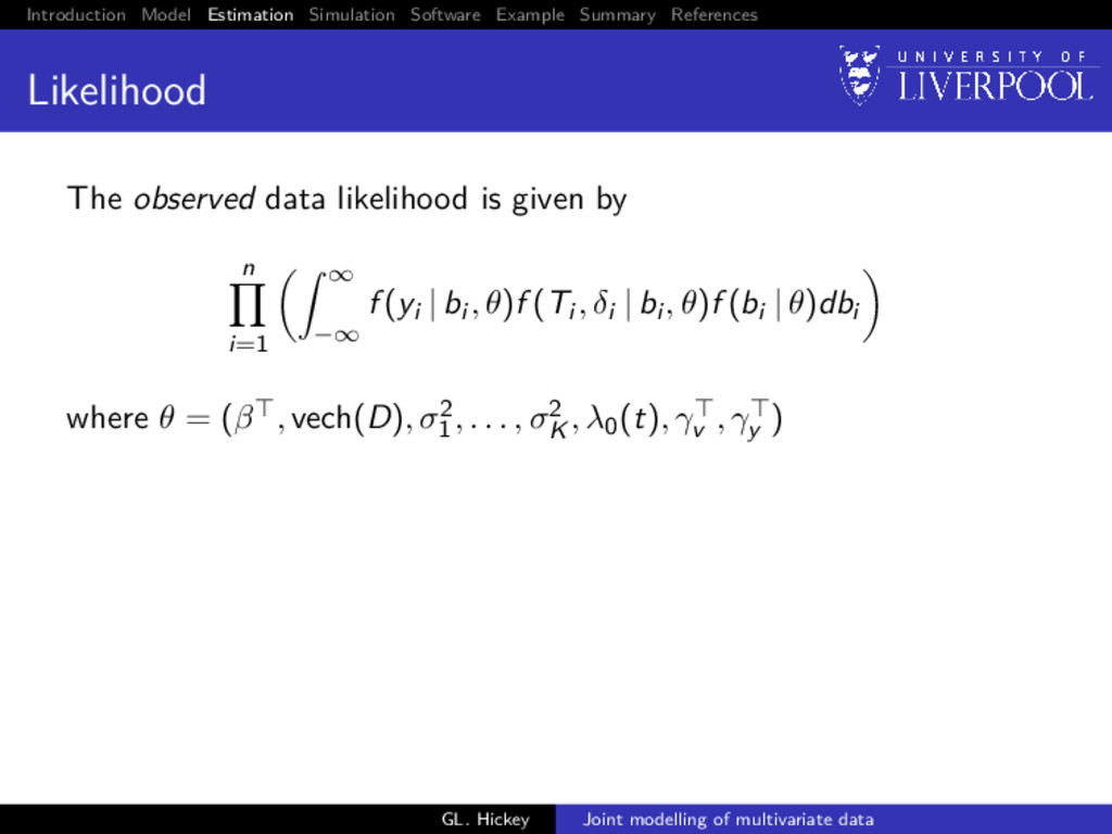
14. Introduction Model Estimation Simulation Software Example Summary References Likelihood The observed data likelihood is given by n i=1 ∞ −∞ f (yi | bi , θ)f (Ti , δi | bi , θ)f (bi | θ)dbi where θ = (β , vech(D), σ2 1 , . . . , σ2 K , λ0(t), γv , γy ) GL. Hickey Joint modelling of multivariate data
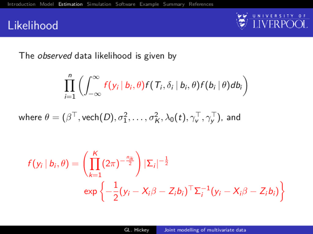
15. Introduction Model Estimation Simulation Software Example Summary References Likelihood The observed data likelihood is given by n i=1 ∞ −∞ f (yi | bi , θ)f (Ti , δi | bi , θ)f (bi | θ)dbi where θ = (β , vech(D), σ2 1 , . . . , σ2 K , λ0(t), γv , γy ), and f (yi | bi , θ) = K k=1 (2π)−nik 2 |Σi |−1 2 exp − 1 2 (yi − Xi β − Zi bi ) Σ−1 i (yi − Xi β − Zi bi ) GL. Hickey Joint modelling of multivariate data
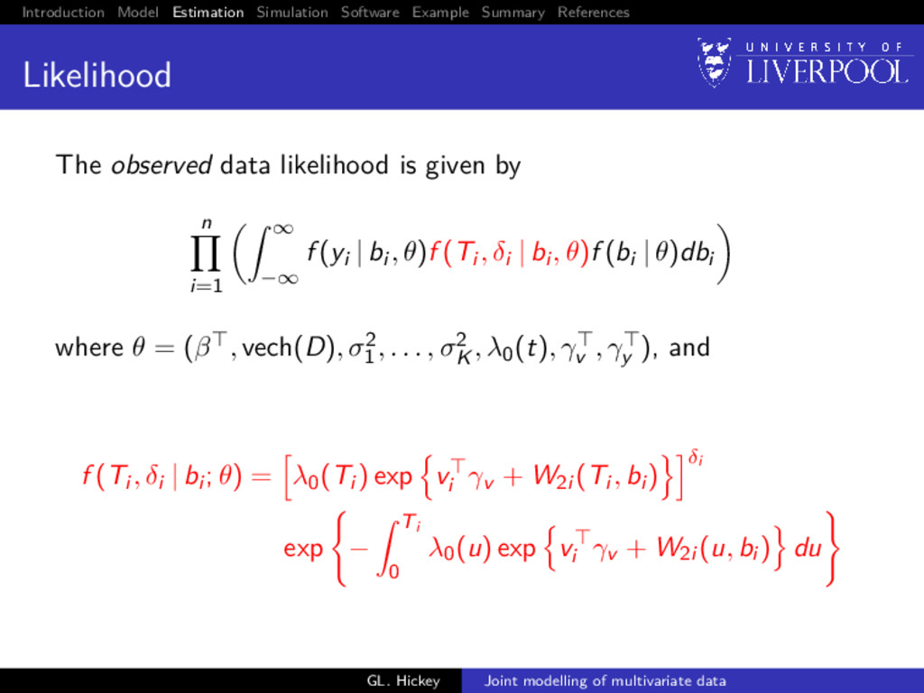
16. Introduction Model Estimation Simulation Software Example Summary References Likelihood The observed data likelihood is given by n i=1 ∞ −∞ f (yi | bi , θ)f (Ti , δi | bi , θ)f (bi | θ)dbi where θ = (β , vech(D), σ2 1 , . . . , σ2 K , λ0(t), γv , γy ), and f (Ti , δi | bi ; θ) = λ0(Ti ) exp vi γv + W2i (Ti , bi ) δi exp − Ti 0 λ0(u) exp vi γv + W2i (u, bi ) du GL. Hickey Joint modelling of multivariate data
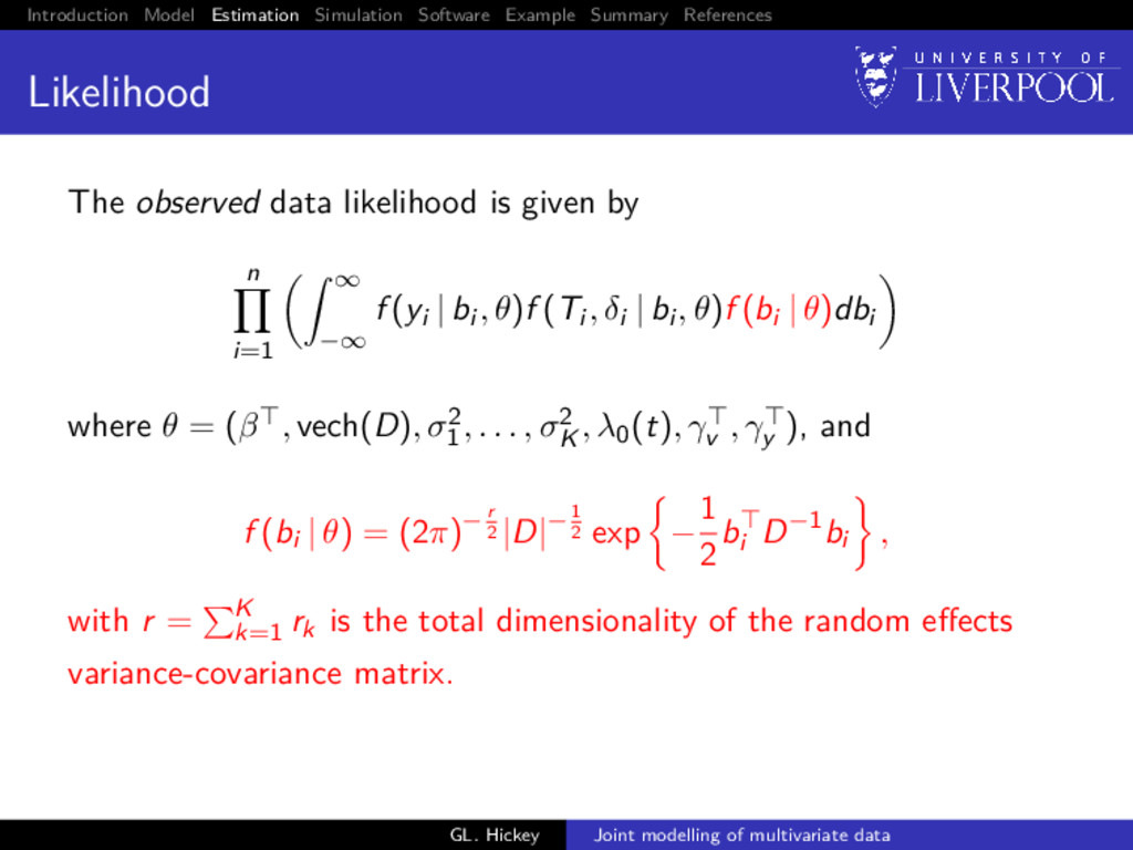
17. Introduction Model Estimation Simulation Software Example Summary References Likelihood The observed data likelihood is given by n i=1 ∞ −∞ f (yi | bi , θ)f (Ti , δi | bi , θ)f (bi | θ)dbi where θ = (β , vech(D), σ2 1 , . . . , σ2 K , λ0(t), γv , γy ), and f (bi | θ) = (2π)− r 2 |D|−1 2 exp − 1 2 bi D−1bi , with r = K k=1 rk is the total dimensionality of the random effects variance-covariance matrix. GL. Hickey Joint modelling of multivariate data
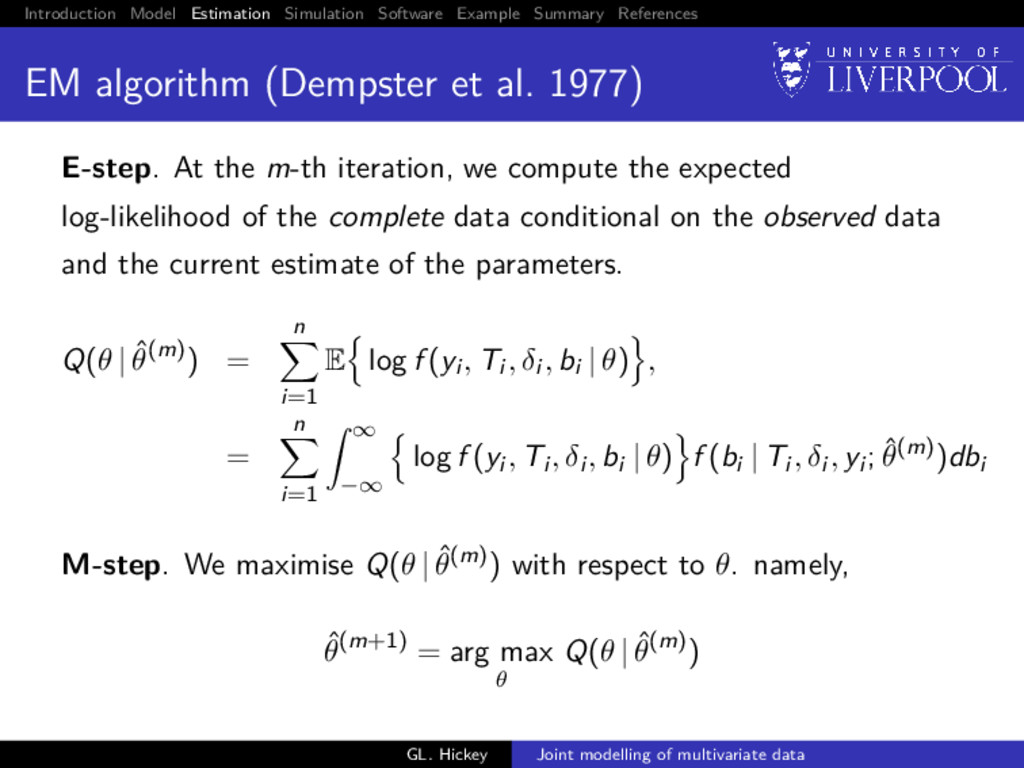
18. Introduction Model Estimation Simulation Software Example Summary References EM algorithm (Dempster et al. 1977) E-step. At the m-th iteration, we compute the expected log-likelihood of the complete data conditional on the observed data and the current estimate of the parameters. Q(θ | ˆ θ(m)) = n i=1 E log f (yi , Ti , δi , bi | θ) , = n i=1 ∞ −∞ log f (yi , Ti , δi , bi | θ) f (bi | Ti , δi , yi ; ˆ θ(m))dbi GL. Hickey Joint modelling of multivariate data
19. Introduction Model Estimation Simulation Software Example Summary References EM algorithm (Dempster et al. 1977) E-step. At the m-th iteration, we compute the expected log-likelihood of the complete data conditional on the observed data and the current estimate of the parameters. Q(θ | ˆ θ(m)) = n i=1 E log f (yi , Ti , δi , bi | θ) , = n i=1 ∞ −∞ log f (yi , Ti , δi , bi | θ) f (bi | Ti , δi , yi ; ˆ θ(m))dbi M-step. We maximise Q(θ | ˆ θ(m)) with respect to θ. namely, ˆ θ(m+1) = arg max θ Q(θ | ˆ θ(m)) GL. Hickey Joint modelling of multivariate data
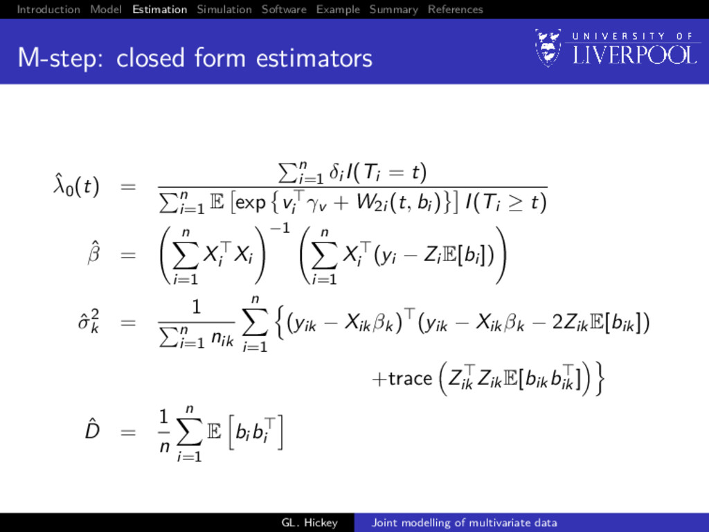
20. Introduction Model Estimation Simulation Software Example Summary References M-step: closed form estimators ˆ λ0(t) = n i=1 δi I(Ti = t) n i=1 E exp vi γv + W2i (t, bi ) I(Ti ≥ t) ˆ β = n i=1 Xi Xi −1 n i=1 Xi (yi − Zi E[bi ]) ˆ σ2 k = 1 n i=1 nik n i=1 (yik − Xikβk) (yik − Xikβk − 2ZikE[bik]) +trace Zik ZikE[bikbik ] ˆ D = 1 n n i=1 E bi bi GL. Hickey Joint modelling of multivariate data
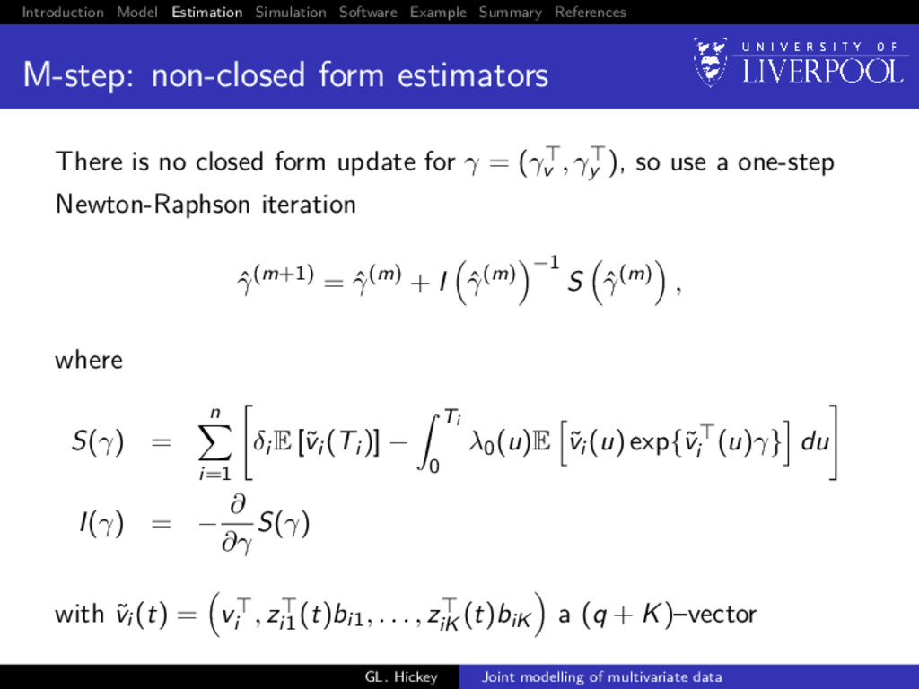
21. Introduction Model Estimation Simulation Software Example Summary References M-step: non-closed form estimators There is no closed form update for γ = (γv , γy ), so use a one-step Newton-Raphson iteration ˆ γ(m+1) = ˆ γ(m) + I ˆ γ(m) −1 S ˆ γ(m) , where S(γ) = n i=1 δi E [˜ vi (Ti )] − Ti 0 λ0(u)E ˜ vi (u) exp{˜ vi (u)γ} du I(γ) = − ∂ ∂γ S(γ) with ˜ vi (t) = vi , zi1 (t)bi1, . . . , ziK (t)biK a (q + K)–vector GL. Hickey Joint modelling of multivariate data
22. Introduction Model Estimation Simulation Software Example Summary References M-step: non-closed form estimators Calculation of I(γ) is the computational bottleneck of the estimation algorithm computation time O(DJ2) (D = number of MC samples; J = number of unique failure times) Accounts for 76% of algorithm time in typical example problem Possible solution: use a Gauss-Newton-like approximation for I(γ)? GL. Hickey Joint modelling of multivariate data
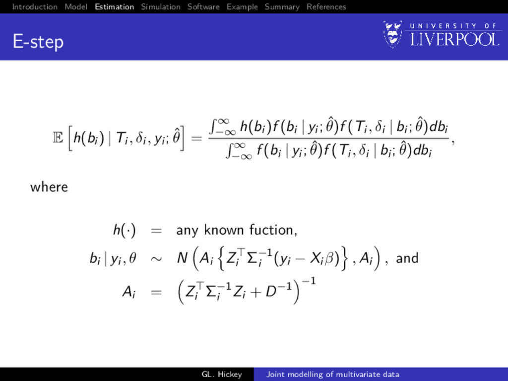
23. Introduction Model Estimation Simulation Software Example Summary References E-step E h(bi ) | Ti , δi , yi ; ˆ θ = ∞ −∞ h(bi )f (bi | yi ; ˆ θ)f (Ti , δi | bi ; ˆ θ)dbi ∞ −∞ f (bi | yi ; ˆ θ)f (Ti , δi | bi ; ˆ θ)dbi , where h(·) = any known fuction, bi | yi , θ ∼ N Ai Zi Σ−1 i (yi − Xi β) , Ai , and Ai = Zi Σ−1 i Zi + D−1 −1 GL. Hickey Joint modelling of multivariate data
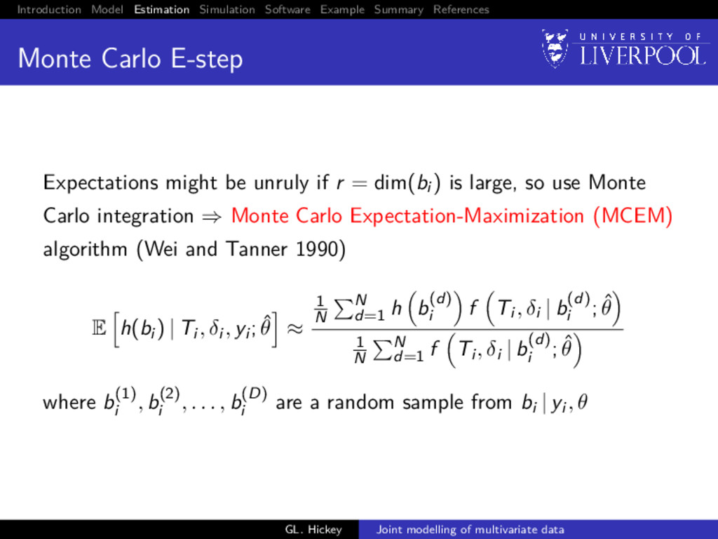
24. Introduction Model Estimation Simulation Software Example Summary References Monte Carlo E-step Expectations might be unruly if r = dim(bi ) is large, so use Monte Carlo integration ⇒ Monte Carlo Expectation-Maximization (MCEM) algorithm (Wei and Tanner 1990) E h(bi ) | Ti , δi , yi ; ˆ θ ≈ 1 N N d=1 h b(d) i f Ti , δi | b(d) i ; ˆ θ 1 N N d=1 f Ti , δi | b(d) i ; ˆ θ where b(1) i , b(2) i , . . . , b(D) i are a random sample from bi | yi , θ GL. Hickey Joint modelling of multivariate data
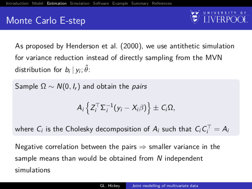
25. Introduction Model Estimation Simulation Software Example Summary References Monte Carlo E-step As proposed by Henderson et al. (2000), we use antithetic simulation for variance reduction instead of directly sampling from the MVN distribution for bi | yi ; ˆ θ: Sample Ω ∼ N(0, Ir ) and obtain the pairs Ai Zi Σ−1 i (yi − Xi β) ± Ci Ω, where Ci is the Cholesky decomposition of Ai such that Ci Ci = Ai Negative correlation between the pairs ⇒ smaller variance in the sample means than would be obtained from N independent simulations GL. Hickey Joint modelling of multivariate data
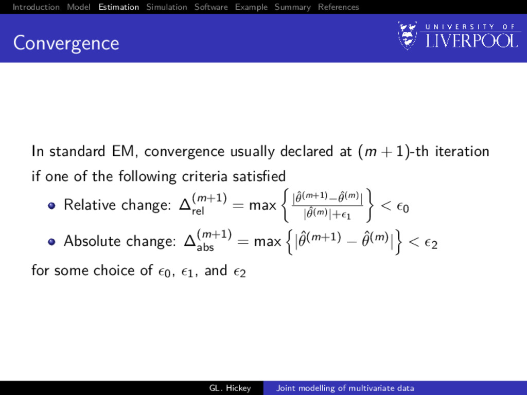
26. Introduction Model Estimation Simulation Software Example Summary References Convergence In standard EM, convergence usually declared at (m + 1)-th iteration if one of the following criteria satisfied Relative change: ∆(m+1) rel = max |ˆ θ(m+1)−ˆ θ(m)| |ˆ θ(m)|+ 1 < 0 Absolute change: ∆(m+1) abs = max |ˆ θ(m+1) − ˆ θ(m)| < 2 for some choice of 0, 1, and 2 GL. Hickey Joint modelling of multivariate data
27. Introduction Model Estimation Simulation Software Example Summary References Convergence In MCEM framework, there are 2 complications to account for GL. Hickey Joint modelling of multivariate data
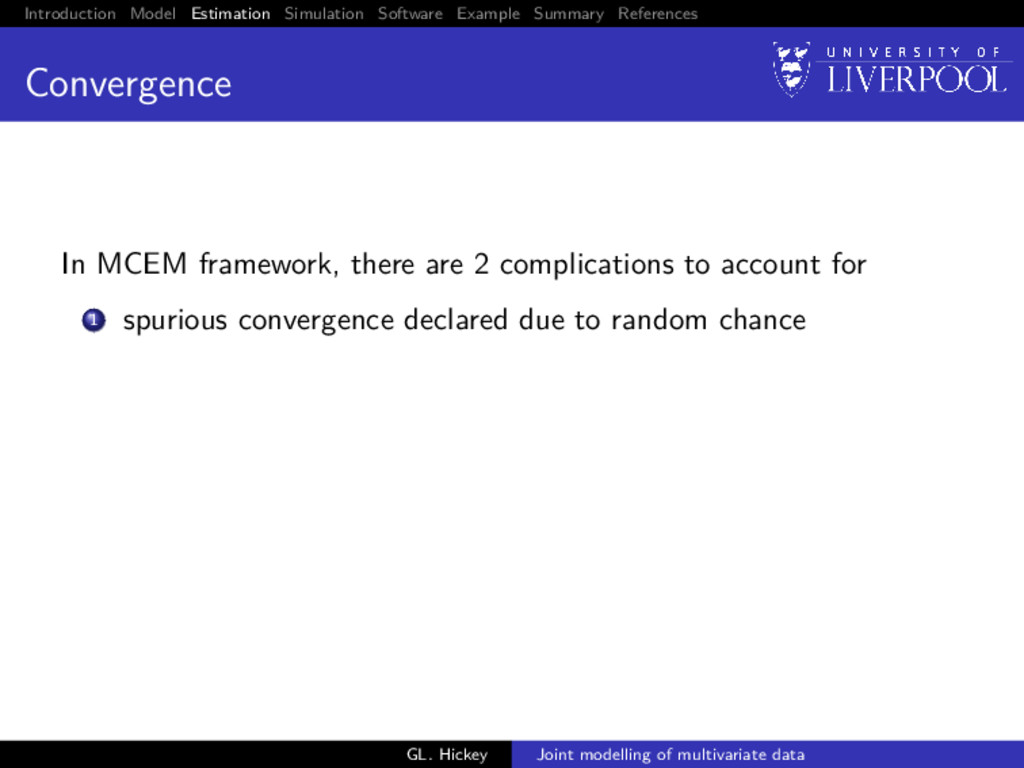
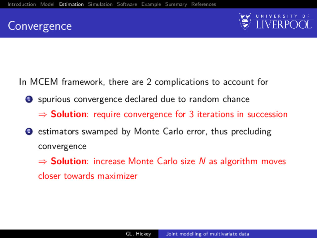
28. Introduction Model Estimation Simulation Software Example Summary References Convergence In MCEM framework, there are 2 complications to account for 1 spurious convergence declared due to random chance GL. Hickey Joint modelling of multivariate data
29. Introduction Model Estimation Simulation Software Example Summary References Convergence In MCEM framework, there are 2 complications to account for 1 spurious convergence declared due to random chance ⇒ Solution: require convergence for 3 iterations in succession GL. Hickey Joint modelling of multivariate data
30. Introduction Model Estimation Simulation Software Example Summary References Convergence In MCEM framework, there are 2 complications to account for 1 spurious convergence declared due to random chance ⇒ Solution: require convergence for 3 iterations in succession 2 estimators swamped by Monte Carlo error, thus precluding convergence GL. Hickey Joint modelling of multivariate data
31. Introduction Model Estimation Simulation Software Example Summary References Convergence In MCEM framework, there are 2 complications to account for 1 spurious convergence declared due to random chance ⇒ Solution: require convergence for 3 iterations in succession 2 estimators swamped by Monte Carlo error, thus precluding convergence ⇒ Solution: increase Monte Carlo size N as algorithm moves closer towards maximizer GL. Hickey Joint modelling of multivariate data
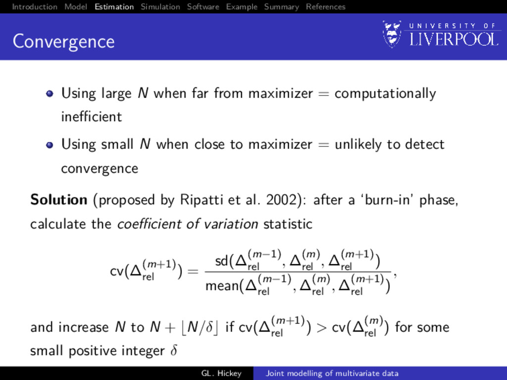
32. Introduction Model Estimation Simulation Software Example Summary References Convergence Using large N when far from maximizer = computationally inefficient Using small N when close to maximizer = unlikely to detect convergence Solution (proposed by Ripatti et al. 2002): after a ‘burn-in’ phase, calculate the coefficient of variation statistic cv(∆(m+1) rel ) = sd(∆(m−1) rel , ∆(m) rel , ∆(m+1) rel ) mean(∆(m−1) rel , ∆(m) rel , ∆(m+1) rel ) , and increase N to N + N/δ if cv(∆(m+1) rel ) > cv(∆(m) rel ) for some small positive integer δ GL. Hickey Joint modelling of multivariate data
33. Introduction Model Estimation Simulation Software Example Summary References Standard error estimation There are two approaches available: GL. Hickey Joint modelling of multivariate data
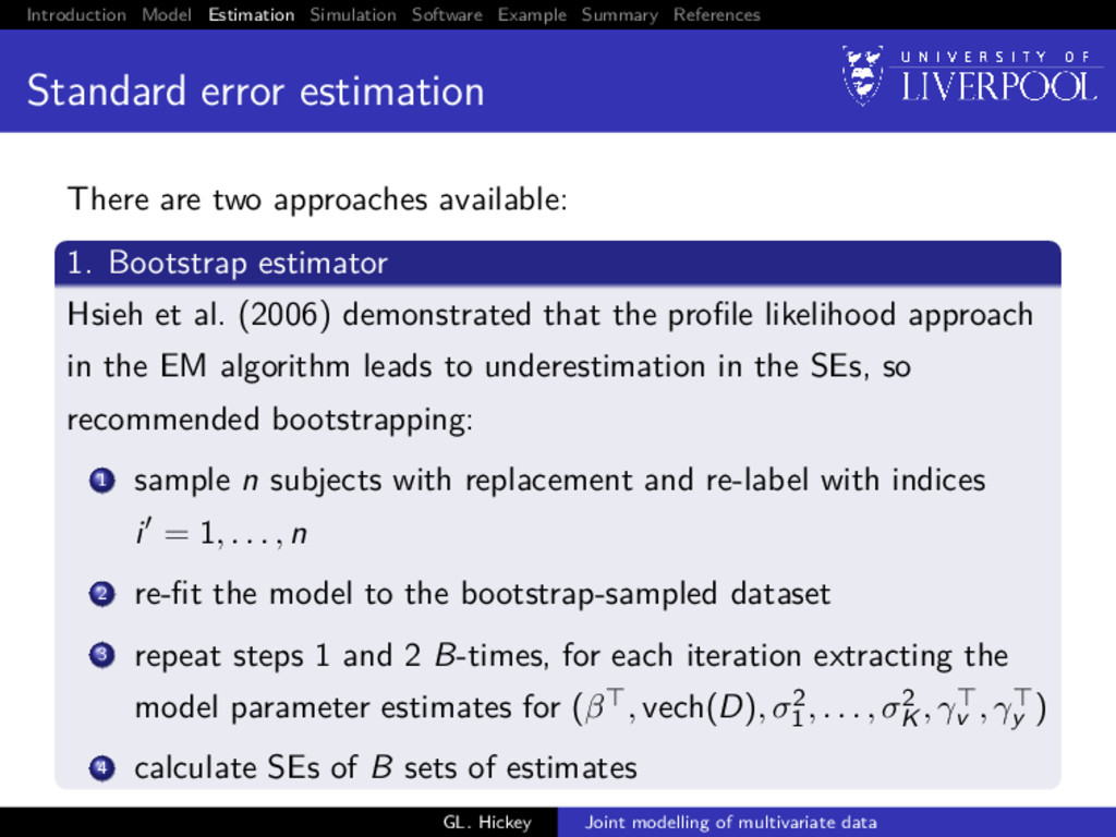
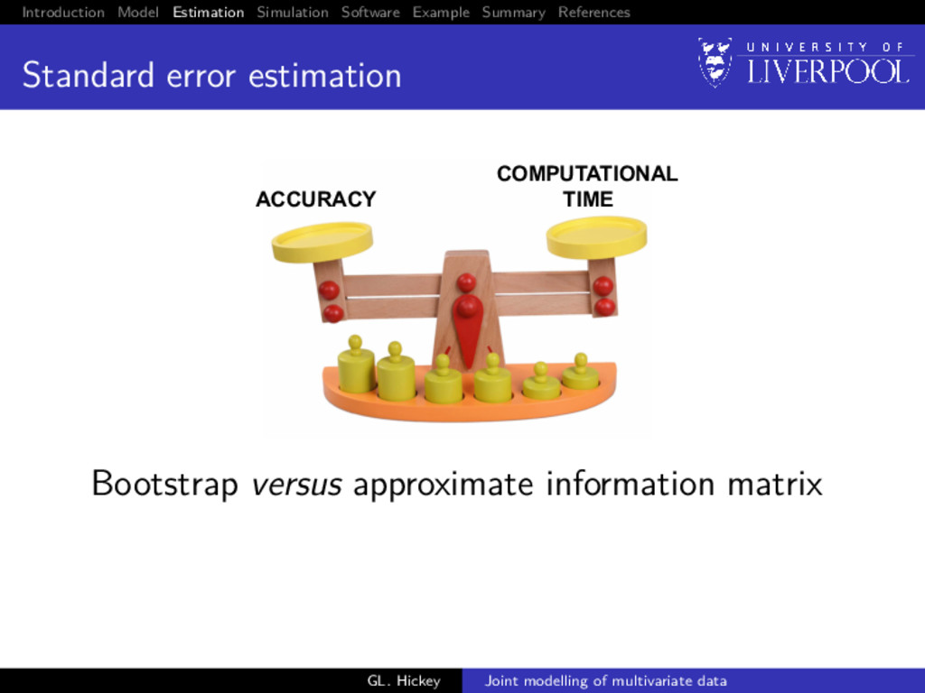
34. Introduction Model Estimation Simulation Software Example Summary References Standard error estimation There are two approaches available: 1. Bootstrap estimator Hsieh et al. (2006) demonstrated that the profile likelihood approach in the EM algorithm leads to underestimation in the SEs, so recommended bootstrapping: 1 sample n subjects with replacement and re-label with indices i = 1, . . . , n 2 re-fit the model to the bootstrap-sampled dataset 3 repeat steps 1 and 2 B-times, for each iteration extracting the model parameter estimates for (β , vech(D), σ2 1 , . . . , σ2 K , γv , γy ) 4 calculate SEs of B sets of estimates GL. Hickey Joint modelling of multivariate data
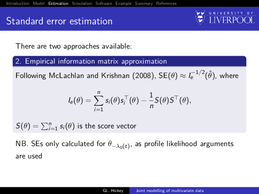
35. Introduction Model Estimation Simulation Software Example Summary References Standard error estimation There are two approaches available: 2. Empirical information matrix approximation Following McLachlan and Krishnan (2008), SE(θ) ≈ I−1/2 e (ˆ θ), where Ie(θ) = n i=1 si (θ)si (θ) − 1 n S(θ)S (θ), S(θ) = n i=1 si (θ) is the score vector NB. SEs only calculated for θ−λ0(t) , as profile likelihood arguments are used GL. Hickey Joint modelling of multivariate data
36. Introduction Model Estimation Simulation Software Example Summary References Standard error estimation ACCURACY COMPUTATIONAL TIME Bootstrap versus approximate information matrix GL. Hickey Joint modelling of multivariate data
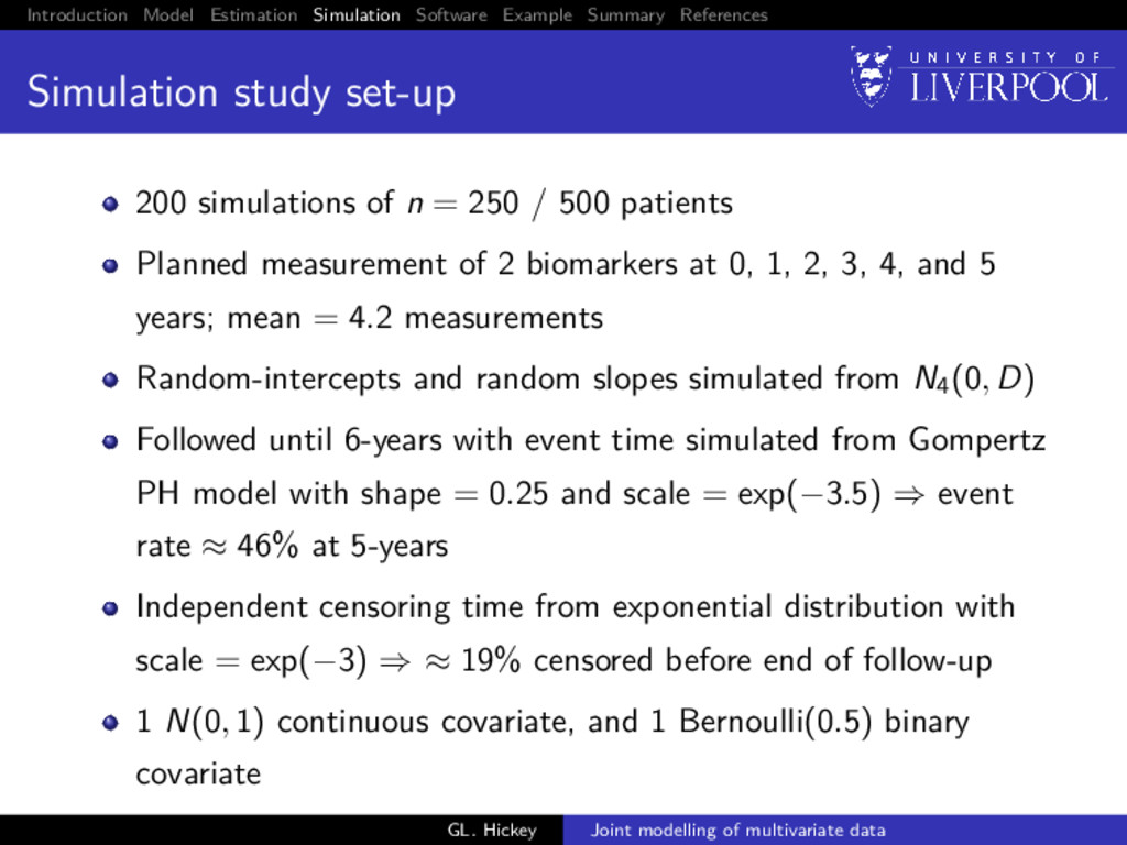
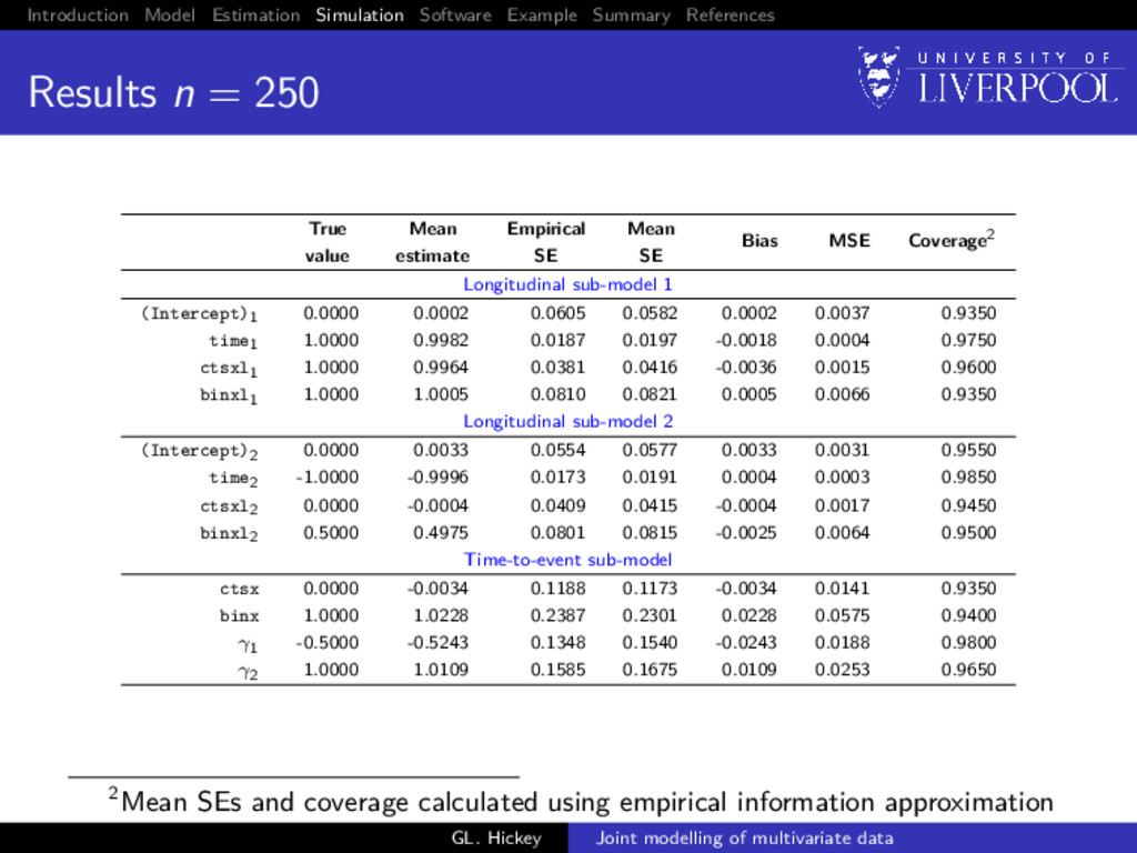
37. Introduction Model Estimation Simulation Software Example Summary References Simulation study set-up 200 simulations of n = 250 / 500 patients Planned measurement of 2 biomarkers at 0, 1, 2, 3, 4, and 5 years; mean = 4.2 measurements Random-intercepts and random slopes simulated from N4(0, D) Followed until 6-years with event time simulated from Gompertz PH model with shape = 0.25 and scale = exp(−3.5) ⇒ event rate ≈ 46% at 5-years Independent censoring time from exponential distribution with scale = exp(−3) ⇒ ≈ 19% censored before end of follow-up 1 N(0, 1) continuous covariate, and 1 Bernoulli(0.5) binary covariate GL. Hickey Joint modelling of multivariate data
38. Introduction Model Estimation Simulation Software Example Summary References Results n = 250 True value Mean estimate Empirical SE Mean SE Bias MSE Coverage2 Longitudinal sub-model 1 (Intercept)1 0.0000 0.0002 0.0605 0.0582 0.0002 0.0037 0.9350 time1 1.0000 0.9982 0.0187 0.0197 -0.0018 0.0004 0.9750 ctsxl1 1.0000 0.9964 0.0381 0.0416 -0.0036 0.0015 0.9600 binxl1 1.0000 1.0005 0.0810 0.0821 0.0005 0.0066 0.9350 Longitudinal sub-model 2 (Intercept)2 0.0000 0.0033 0.0554 0.0577 0.0033 0.0031 0.9550 time2 -1.0000 -0.9996 0.0173 0.0191 0.0004 0.0003 0.9850 ctsxl2 0.0000 -0.0004 0.0409 0.0415 -0.0004 0.0017 0.9450 binxl2 0.5000 0.4975 0.0801 0.0815 -0.0025 0.0064 0.9500 Time-to-event sub-model ctsx 0.0000 -0.0034 0.1188 0.1173 -0.0034 0.0141 0.9350 binx 1.0000 1.0228 0.2387 0.2301 0.0228 0.0575 0.9400 γ1 -0.5000 -0.5243 0.1348 0.1540 -0.0243 0.0188 0.9800 γ2 1.0000 1.0109 0.1585 0.1675 0.0109 0.0253 0.9650 2Mean SEs and coverage calculated using empirical information approximation GL. Hickey Joint modelling of multivariate data
39. Introduction Model Estimation Simulation Software Example Summary References Results n = 500 True value Mean estimate Empirical SE Mean SE Bias MSE Coverage3 Longitudinal sub-model 1 (Intercept)1 0.0000 -0.0022 0.0376 0.0402 -0.0022 0.0014 0.9600 time1 1.0000 1.0001 0.0129 0.0137 0.0001 0.0002 0.9750 ctsxl1 1.0000 0.9959 0.0243 0.0285 -0.0041 0.0006 0.9700 binxl1 1.0000 1.0045 0.0527 0.0564 0.0045 0.0028 0.9600 Longitudinal sub-model 2 (Intercept)2 0.0000 0.0017 0.0352 0.0400 0.0017 0.0012 0.9600 time2 -1.0000 -0.9992 0.0135 0.0131 0.0008 0.0002 0.9350 ctsxl2 0.0000 0.0013 0.0269 0.0284 0.0013 0.0007 0.9500 binxl2 0.5000 0.4973 0.0526 0.0563 -0.0027 0.0028 0.9750 Time-to-event sub-model ctsx 0.0000 0.0104 0.0791 0.0789 0.0104 0.0064 0.9550 binx 1.0000 0.9952 0.1627 0.1571 -0.0048 0.0265 0.9300 γ1 -0.5000 -0.4976 0.0987 0.1006 0.0024 0.0098 0.9700 γ2 1.0000 1.0061 0.1045 0.1091 0.0061 0.0109 0.9500 3Mean SEs and coverage calculated using empirical information approximation GL. Hickey Joint modelling of multivariate data
40. Introduction Model Estimation Simulation Software Example Summary References joineRML An R package is now available for fitting this model: joineRML Currently on GitHub (due for CRAN submission shortly): github.com/graemeleehickey/joineRML Complements existing R package for univariate joint models: joineR (available on CRAN) GL. Hickey Joint modelling of multivariate data
41. Introduction Model Estimation Simulation Software Example Summary References Example code GL. Hickey Joint modelling of multivariate data
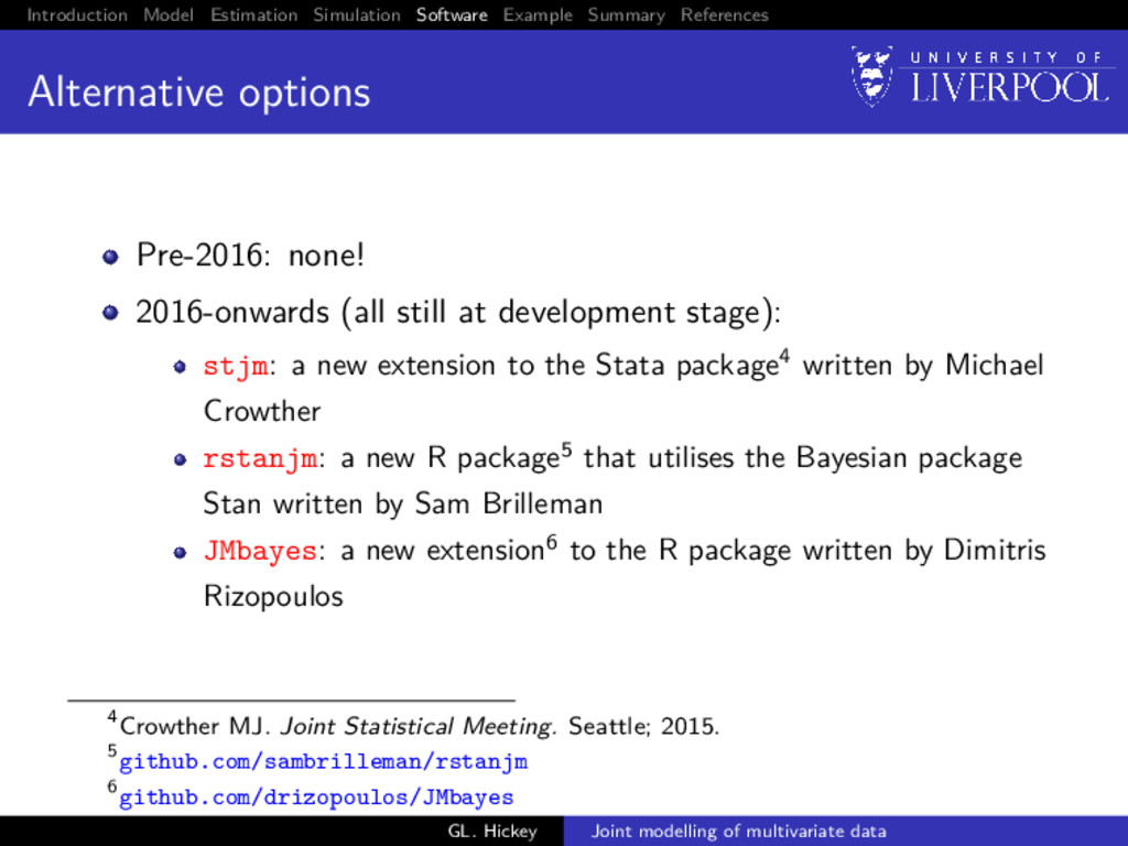
42. Introduction Model Estimation Simulation Software Example Summary References Alternative options Pre-2016: none! 2016-onwards (all still at development stage): stjm: a new extension to the Stata package4 written by Michael Crowther rstanjm: a new R package5 that utilises the Bayesian package Stan written by Sam Brilleman JMbayes: a new extension6 to the R package written by Dimitris Rizopoulos 4Crowther MJ. Joint Statistical Meeting. Seattle; 2015. 5 github.com/sambrilleman/rstanjm 6 github.com/drizopoulos/JMbayes GL. Hickey Joint modelling of multivariate data
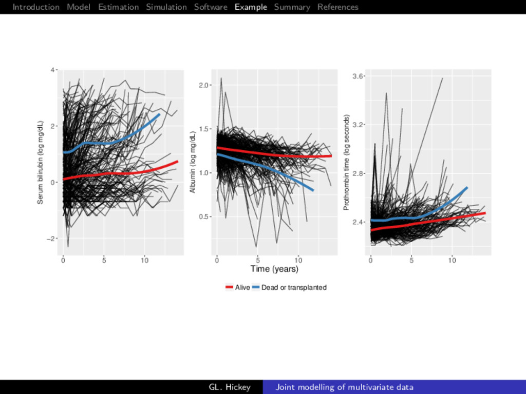
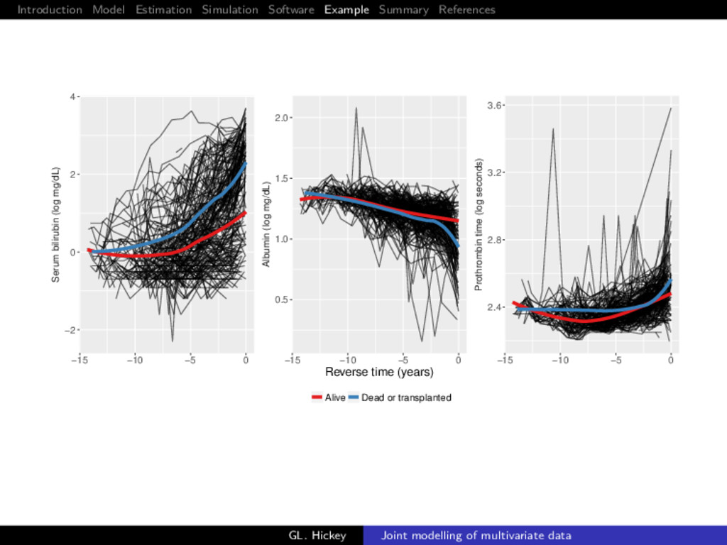
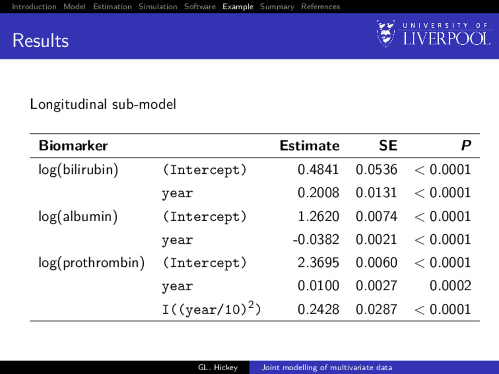
43. Introduction Model Estimation Simulation Software Example Summary References The Mayo Clinic PBC data Primary biliary cirrhosis (PBC) is a chronic liver disease characterized by inflammatory destruction of the small bile ducts, which eventually leads to cirrhosis of the liver (Murtaugh et al. 1994) Trial conducted between 1974 and 1984 randomized 312 patients to either placebo or D-penicillamine Multiple biomarkers repeatedly measured at intermittent times: 1 serum bilirunbin (mg/dl) 2 serum albumin (mg/dl) 3 prothrombin time (seconds) Time to death or transplantation (competing risks) GL. Hickey Joint modelling of multivariate data
44. Introduction Model Estimation Simulation Software Example Summary References Prothrombin time (log seconds) Albumin (log mg/dL) Serum bilirubin (log mg/dL) 0 5 10 0 5 10 0 5 10 2.4 2.8 3.2 3.6 0.5 1.0 1.5 2.0 −2 0 2 4 Time (years) Alive Dead or transplanted GL. Hickey Joint modelling of multivariate data
45. Introduction Model Estimation Simulation Software Example Summary References Prothrombin time (log seconds) Albumin (log mg/dL) Serum bilirubin (log mg/dL) −15 −10 −5 0 −15 −10 −5 0 −15 −10 −5 0 2.4 2.8 3.2 3.6 0.5 1.0 1.5 2.0 −2 0 2 4 Reverse time (years) Alive Dead or transplanted GL. Hickey Joint modelling of multivariate data
46. Introduction Model Estimation Simulation Software Example Summary References 0 2 4 6 8 10 12 14 0.0 0.2 0.4 0.6 0.8 1.0 Time from registration Freedom from death or transplantation GL. Hickey Joint modelling of multivariate data
47. Introduction Model Estimation Simulation Software Example Summary References Proposed model Longitudinal sub-model log(bil) = (β0,1 + b0i,1) + (β1,1 + b1i,1)year + εij1, log(alb) = (β0,2 + b0i,2) + (β1,2 + b1i,2)year + εij2, log(pro) = (β0,3 + b0i,3) + (β1,3 + b1i,3)year + β2,3(year/10)2 + εij3, bi ∼ N6(0, D), and εijk ∼ N(0, σ2 k ) for k = 1, 2, 3 Time-to-event sub-model λi (t) = λ0(t) exp {γv age + W2i (t)} W2i (t) = γbil (b0i,1 + b1i,1t) + γalb (b0i,2 + b1i,2t) + γpro (b0i,3 + b1i,3t) GL. Hickey Joint modelling of multivariate data
48. Introduction Model Estimation Simulation Software Example Summary References Results Longitudinal sub-model Biomarker Estimate SE P log(bilirubin) (Intercept) 0.4841 0.0536 < 0.0001 year 0.2008 0.0131 < 0.0001 log(albumin) (Intercept) 1.2620 0.0074 < 0.0001 year -0.0382 0.0021 < 0.0001 log(prothrombin) (Intercept) 2.3695 0.0060 < 0.0001 year 0.0100 0.0027 0.0002 I((year/10)2) 0.2428 0.0287 < 0.0001 GL. Hickey Joint modelling of multivariate data
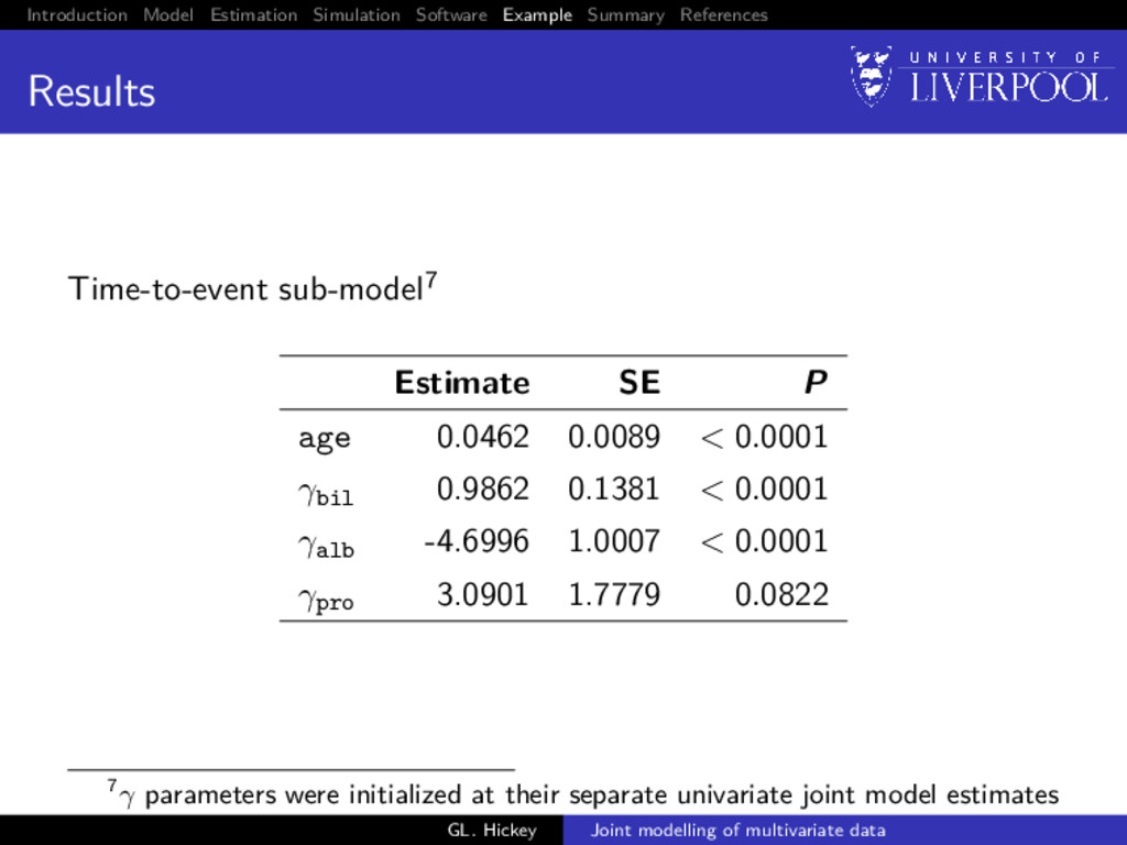
49. Introduction Model Estimation Simulation Software Example Summary References Results Time-to-event sub-model7 Estimate SE P age 0.0462 0.0089 < 0.0001 γbil 0.9862 0.1381 < 0.0001 γalb -4.6996 1.0007 < 0.0001 γpro 3.0901 1.7779 0.0822 7γ parameters were initialized at their separate univariate joint model estimates GL. Hickey Joint modelling of multivariate data
50. Introduction Model Estimation Simulation Software Example Summary References Future research Develop joineRML package to be faster and more accurate Extend to include competing risks and recurrent events; e.g. Williamson et al. (2008) Incorporate model diagnostics; e.g. residuals GL. Hickey Joint modelling of multivariate data
51. Introduction Model Estimation Simulation Software Example Summary References Acknowledgements Project investigators: Dr. Ruwanthi Kolamunnage-Dona (University of Liverpool) Dr. Pete Philipson (University of Northumbria) Dr. Andrea Jorgensen (University of Liverpool) Statistical collaborators: Prof. Robin Henderson (University of Newcastle) Prof. Paula Williamson (University of Liverpool) Funding: Medical Research Council (MR/M013227/1) GL. Hickey Joint modelling of multivariate data
52. Introduction Model Estimation Simulation Software Example Summary References References I Hickey, GL et al. (2016). Joint modelling of time-to-event and multivariate longitudinal outcomes: recent developments and issues. BMC Med Res Meth 16(1), pp. 1–15. Laird, NM and Ware, JH (1982). Random-effects models for longitudinal data. Biometrics 38(4), pp. 963–74. Henderson, R et al. (2000). Joint modelling of longitudinal measurements and event time data. Biostatistics 1(4), pp. 465–480. Wulfsohn, MS and Tsiatis, AA (1997). A joint model for survival and longitudinal data measured with error. Biometrics 53(1), pp. 330–339. Lin, H et al. (2002). Maximum likelihood estimation in the joint analysis of time-to-event and multiple longitudinal variables. Stat Med 21, pp. 2369–2382. Dempster, AP et al. (1977). Maximum likelihood from incomplete data via the EM algorithm. J Roy Stat Soc B 39(1), pp. 1–38. GL. Hickey Joint modelling of multivariate data
53. Introduction Model Estimation Simulation Software Example Summary References References II Wei, GC and Tanner, MA (1990). A Monte Carlo implementation of the EM algorithm and the poor man’s data augmentation algorithms. J Am Stat Assoc 85(411), pp. 699–704. Ripatti, S et al. (2002). Maximum likelihood inference for multivariate frailty models using an automated Monte Carlo EM algorithm. Life Dat Anal 8(2002), pp. 349–360. Hsieh, F et al. (2006). Joint modeling of survival and longitudinal data: Likelihood approach revisited. Biometrics 62(4), pp. 1037–1043. McLachlan, GJ and Krishnan, T (2008). The EM Algorithm and Extensions. Second. Wiley-Interscience. Murtaugh, Paul A et al. (1994). Primary biliary cirrhosis: prediction of short-term survival based on repeated patient visits. Hepatology 20(1), pp. 126–134. Williamson, Paula R et al. (2008). Joint modelling of longitudinal and competing risks data. Statistics in Medicine 27, pp. 6426–6438. GL. Hickey Joint modelling of multivariate data