Joint modelling of multivariate longitudinal and time-to-event data

Research into joint modelling methods has grown substantially over recent years. Previous research has predominantly concentrated on the joint modelling of a single longitudinal outcome and a single time-to-event outcome. In clinical practice, the data collected will often be more complex, featuring multiple longitudinal outcomes and/or multiple, recurrent or competing event times. Harnessing all available measurements in a single model is advantageous and should lead to improved and more specific model predictions.

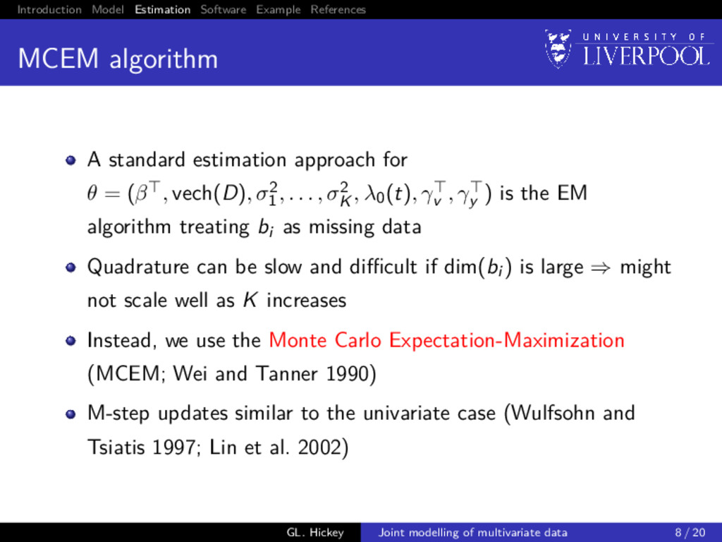
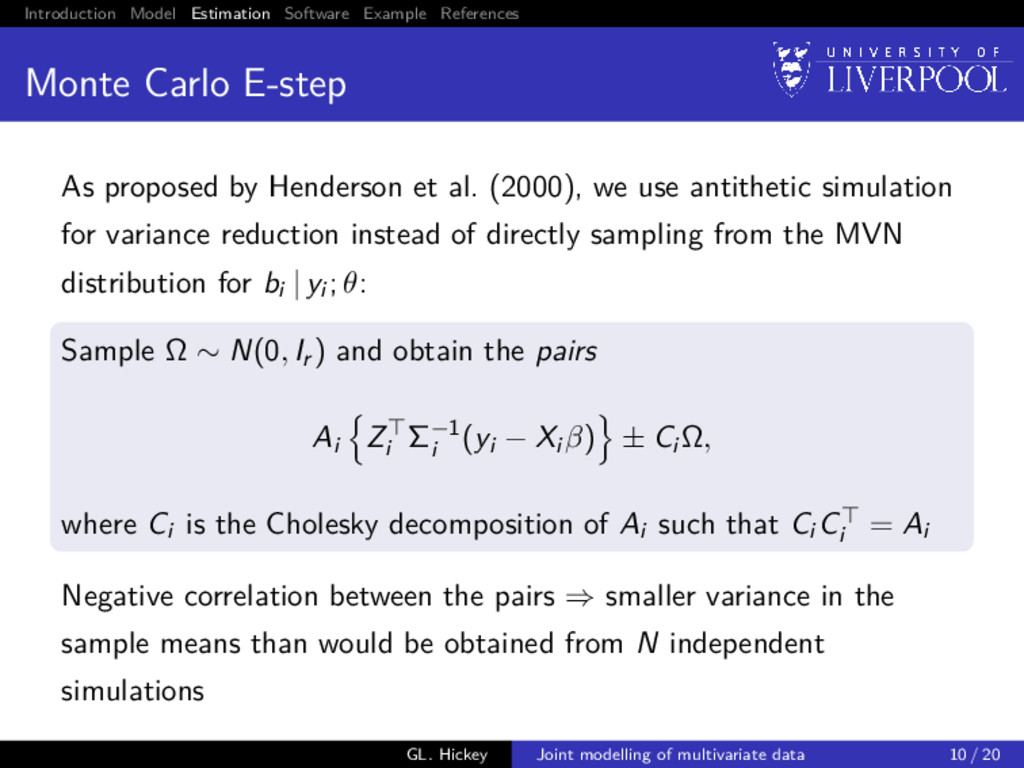
Notwithstanding the increased flexibility and better predictive capabilities, the extension of the classical univariate joint modelling framework to a multivariate setting introduces a number of technical and computational challenges. These include the high-dimensional numerical integrations required, modelling of multivariate unbalanced data, and proper estimation of standard errors. Consequently, software capable of fitting joint models to multivariate data is lacking. Building on recent methodological developments, we extend the classical joint model to multiple continuous longitudinal outcomes, and describe how to fit it using a Monte Carlo Expectation-Maximization algorithm with antithetic simulation for variance reduction. The development of a new R package, joineRML (https://CRAN.R-project.org/package=joineRML), will be demonstrated and an application to a clinical trial dataset will be presented.

Transcript

1. Introduction Model Estimation Software Example References Joint modelling of multivariate longitudinal and time-to-event data Graeme L. Hickey1, Pete Philipson2, Andrea Jorgensen1, Ruwanthi-Kolamunnage-Dona1 1Department of Biostatistics, University of Liverpool, UK 2Mathematics, Physics and Electrical Engineering, University of Northumbria, UK graeme.hickey@liverpool.ac.uk 3rd July 2017 GL. Hickey Joint modelling of multivariate data 1 / 20
2. Introduction Model Estimation Software Example References Motivation for multivariate joint models Clinical studies often repeatedly measure multiple biomarkers or other measurements and an event time As of 2015: > 200 methodological papers and > 60 clinical applications of joint models (Sudell et al. 2016) Many software packages available for univariate models, but not for multivariate models (Hickey et al. 2016) ⇒ limits many applied statisticians to univariate models only GL. Hickey Joint modelling of multivariate data 2 / 20
3. Introduction Model Estimation Software Example References Motivation for multivariate joint models Clinical studies often repeatedly measure multiple biomarkers or other measurements and an event time As of 2015: > 200 methodological papers and > 60 clinical applications of joint models (Sudell et al. 2016) Many software packages available for univariate models, but not for multivariate models (Hickey et al. 2016) ⇒ limits many applied statisticians to univariate models only Objective Develop an package that extends the existing capabilities of joineR GL. Hickey Joint modelling of multivariate data 2 / 20
4. Introduction Model Estimation Software Example References Data For each subject i = 1, . . . , n, we observe yi = (yi1 , . . . , yiK ) is a K-variate continuous outcome vector, where each yik denotes an (nik × 1)-vector of observed longitudinal measurements for the k-th outcome type: yik = (yi1k, . . . , yinik k) Observation times tijk for j = 1, . . . , nik, which can differ between subjects and outcomes (Ti , δi ), where Ti = min(T∗ i , Ci ), where T∗ i is the true event time, Ci corresponds to a potential right-censoring time, and δi is the failure indicator equal to 1 if the failure is observed (T∗ i ≤ Ci ) and 0 otherwise GL. Hickey Joint modelling of multivariate data 3 / 20
5. Introduction Model Estimation Software Example References Longitudinal sub-model Following Henderson et al. (2000) for the univariate case yi (t) = µi (t) + W1i (t) + εi (t), where εi (t) is the model error term, which is i.i.d. N(0, σ2) and independent of W1i (t) µi (t) = xi (t)β is the mean response xi (t) is a p-vector of (possibly) time-varying covariates with corresponding fixed effect terms β W1i (t) is a zero-mean latent Gaussian process GL. Hickey Joint modelling of multivariate data 4 / 20
6. Introduction Model Estimation Software Example References Longitudinal sub-model We can extend it to K-separate sub-models (with k = 1, . . . , K) yik(t) = µik(t) + W (k) 1i (t) + εik(t), where εik(t) is the model error term, which is i.i.d. N(0, σ2 k ) and independent of W (k) 1i (t) µik(t) = xik (t)βk is the mean response xik(t) is a pk-vector of (possibly) time-varying covariates with corresponding fixed effect terms βk W (k) 1i (t) is a zero-mean latent Gaussian process GL. Hickey Joint modelling of multivariate data 4 / 20
7. Introduction Model Estimation Software Example References Time-to-event sub-model λi (t) = λ0(t) exp vi (t)γv + W2i (t) , where λ0(·) is an unspecified baseline hazard function vi (t) is a q-vector of (possibly) time-varying covariates with corresponding fixed effect terms γv W2i (t) is a zero-mean latent Gaussian process, independent of the censoring process GL. Hickey Joint modelling of multivariate data 5 / 20
8. Introduction Model Estimation Software Example References Correlation Following Laird and Ware (1982): W (k) 1i (t) = zik (t)bik for k = 1, . . . , K GL. Hickey Joint modelling of multivariate data 6 / 20
9. Introduction Model Estimation Software Example References Correlation Following Laird and Ware (1982): W (k) 1i (t) = zik (t)bik for k = 1, . . . , K Three sources of correlation: 1 Within-subject correlation between longitudinal measurements: bik ∼ N(0, Dkk) 2 Between longitudinal outcomes correlation: cov(bik, bil ) = Dkl for k = l 3 Correlation between sub-models1: W2i (t) = K k=1 γykW (k) 1i (t) 1Extends model proposed Henderson et al. 2000, although many other W2i (t) specifications have been proposed in literature GL. Hickey Joint modelling of multivariate data 6 / 20
10. Introduction Model Estimation Software Example References Likelihood We can re-write the longitudinal sub-model as yi | bi , β, Σi ∼ N(Xi β + Zi bi , Σi ), with bi | D ∼ N(0, D), where β = (β1 , . . . , βK ), bi = (bi1 , . . . , biK ) , and Xi =      Xi1 · · · 0 . . . ... . . . 0 · · · XiK      , Zi =      Zi1 · · · 0 . . . ... . . . 0 · · · ZiK      , D =      D11 · · · D1K . . . ... . . . D1K · · · DKK      Σi =      σ2 1 Ini1 · · · 0 . . . ... . . . 0 · · · σ2 K IniK      GL. Hickey Joint modelling of multivariate data 7 / 20
11. Introduction Model Estimation Software Example References MCEM algorithm A standard estimation approach for θ = (β , vech(D), σ2 1 , . . . , σ2 K , λ0(t), γv , γy ) is the EM algorithm treating bi as missing data Quadrature can be slow and difficult if dim(bi ) is large ⇒ might not scale well as K increases Instead, we use the Monte Carlo Expectation-Maximization (MCEM; Wei and Tanner 1990) M-step updates similar to the univariate case (Wulfsohn and Tsiatis 1997; Lin et al. 2002) GL. Hickey Joint modelling of multivariate data 8 / 20
12. Introduction Model Estimation Software Example References Monte Carlo E-step Conventional EM algorithm: use quadrature to compute E h(bi ) | Ti , δi , yi ; ˆ θ = ∞ −∞ h(bi )f (bi | yi ; ˆ θ)f (Ti , δi | bi ; ˆ θ)dbi ∞ −∞ f (bi | yi ; ˆ θ)f (Ti , δi | bi ; ˆ θ)dbi , where h(·) = any known fuction, bi | yi , θ ∼ N Ai Zi Σ−1 i (yi − Xi β) , Ai , and Ai = Zi Σ−1 i Zi + D−1 −1 GL. Hickey Joint modelling of multivariate data 9 / 20
13. Introduction Model Estimation Software Example References Monte Carlo E-step MCEM algorithm E-step: use Monte Carlo integration to compute E h(bi ) | Ti , δi , yi ; ˆ θ ≈ 1 N N d=1 h b(d) i f Ti , δi | b(d) i ; ˆ θ 1 N N d=1 f Ti , δi | b(d) i ; ˆ θ where h(·) = any known fuction, bi | yi , θ ∼ N Ai Zi Σ−1 i (yi − Xi β) , Ai , and Ai = Zi Σ−1 i Zi + D−1 −1 b(1) i , b(2) i , . . . , b(N) i ∼ bi | yi , θ a Monte Carlo draw GL. Hickey Joint modelling of multivariate data 9 / 20
14. Introduction Model Estimation Software Example References Monte Carlo E-step As proposed by Henderson et al. (2000), we use antithetic simulation for variance reduction instead of directly sampling from the MVN distribution for bi | yi ; θ: Sample Ω ∼ N(0, Ir ) and obtain the pairs Ai Zi Σ−1 i (yi − Xi β) ± Ci Ω, where Ci is the Cholesky decomposition of Ai such that Ci Ci = Ai Negative correlation between the pairs ⇒ smaller variance in the sample means than would be obtained from N independent simulations GL. Hickey Joint modelling of multivariate data 10 / 20
15. Introduction Model Estimation Software Example References Convergence The monotonicity property of the EM algorithm is lost in the MCEM algorithm, so we need to increase N at each iteration Problem Using large N when far from maximizer = computationally inefficient Using small N when close to maximizer = unlikely to detect convergence GL. Hickey Joint modelling of multivariate data 11 / 20
16. Introduction Model Estimation Software Example References Convergence The monotonicity property of the EM algorithm is lost in the MCEM algorithm, so we need to increase N at each iteration Solution (Ripatti et al. 2002) After a ‘burn-in’ phase, calculate the coefficient of variation statistic cv(∆(m+1) rel ) = sd(∆(m−1) rel , ∆(m) rel , ∆(m+1) rel ) mean(∆(m−1) rel , ∆(m) rel , ∆(m+1) rel ) , and increase N to N + N/δ if cv(∆(m+1) rel ) > cv(∆(m) rel ) for some small positive integer δ, where ∆(m+1) rel = max |ˆ θ(m+1) − ˆ θ(m)| |ˆ θ(m)| + GL. Hickey Joint modelling of multivariate data 11 / 20
17. Introduction Model Estimation Software Example References Standard error estimation Method 1: Bootstrap Hsieh et al. (2006) demonstrated that the profile likelihood approach in the EM algorithm leads to underestimation in the SEs, so recommended bootstrapping GL. Hickey Joint modelling of multivariate data 12 / 20
18. Introduction Model Estimation Software Example References Standard error estimation Method 1: Bootstrap Hsieh et al. (2006) demonstrated that the profile likelihood approach in the EM algorithm leads to underestimation in the SEs, so recommended bootstrapping Method 2: Empirical information matrix approximation Following McLachlan and Krishnan (2008), SE(θ) ≈ I−1/2 e (ˆ θ), where Ie(θ) = n i=1 si (θ)si (θ) − 1 n S(θ)S (θ), S(θ) = n i=1 si (θ) is the score vector GL. Hickey Joint modelling of multivariate data 12 / 20
19. Introduction Model Estimation Software Example References joineRML joineRML + getVarCov() vcov() fixef() ranef()* AIC() BIC() confint() formula() sampleData() dynSurv()* dynLong()* print() summary() plot() sigma() coef() update() baseHaz() residuals() fitted() logLik() bootSE() Rich collection of associated methods * associated with additional plot methods mjoint() Version 0.2.2 available on CRAN https://cran.r-project.org/web/packages/joineRML/ Developmental version available on GitHub https://github.com/graemeleehickey/joineRML GL. Hickey Joint modelling of multivariate data 13 / 20
20. Introduction Model Estimation Software Example References The Mayo Clinic PBC data Primary biliary cirrhosis (PBC) is a chronic liver disease characterized by inflammatory destruction of the small bile ducts, which eventually leads to cirrhosis of the liver (Murtaugh et al. 1994) We analyse a subset of 154 patients randomized to placebo Multiple biomarkers repeatedly measured at intermittent times: 1 serum bilirunbin (mg/dl) 2 serum albumin (mg/dl) 3 prothrombin time (seconds) Patients drop out if they die GL. Hickey Joint modelling of multivariate data 14 / 20
21. Introduction Model Estimation Software Example References Prothrombin time (0.1 x seconds)−4 Albumin (mg dL) Serum bilirubin (loge mg dL) 0 5 10 0 5 10 0 5 10 0.0 0.5 1.0 1.5 2 4 6 8 −2 0 2 4 Time from registration (years) Alive Dead GL. Hickey Joint modelling of multivariate data 15 / 20
22. Introduction Model Estimation Software Example References 0 2 4 6 8 10 12 14 0.0 0.2 0.4 0.6 0.8 1.0 Time from registration (years) Survival probability nevents = 69, 44.8% GL. Hickey Joint modelling of multivariate data 16 / 20
23. Introduction Model Estimation Software Example References Proposed model for PBC data Longitudinal sub-model log(serBilir) = (β0,1 + b0i,1) + (β1,1 + b1i,1)year + εij1, albumin = (β0,2 + b0i,2) + (β1,2 + b1i,2)year + εij2, (0.1 × prothrombin)−4 = (β0,3 + b0i,3) + (β1,3 + b1i,3)year + εij3, bi ∼ N6(0, D), and εijk ∼ N(0, σ2 k ) for k = 1, 2, 3 Time-to-event sub-model λi (t) = λ0(t) exp {γv age + W2i (t)} , W2i (t) = γbil (b0i,1 + b1i,1t) + γalb (b0i,2 + b1i,2t) + γpro (b0i,3 + b1i,3t). GL. Hickey Joint modelling of multivariate data 17 / 20
24. Introduction Model Estimation Software Example References Example code data(pbc2) placebo <- subset(pbc2, drug == "placebo") fit.pbc <- mjoint( formLongFixed = list( "bil" = log(serBilir) ˜ year, "alb" = albumin ˜ year, "pro" = (0.1 * prothrombin)ˆ-4 ˜ year), formLongRandom = list( "bil" = ˜ year | id, "alb" = ˜ year | id, "pro" = ˜ year | id), formSurv = Surv(years, status2) ˜ age, data = placebo, timeVar = "year", control = list(tol0 = 0.001, burin = 400)) GL. Hickey Joint modelling of multivariate data 18 / 20
25. Introduction Model Estimation Software Example References Results Parameter Estimate SE 95% CI β0,1 0.5541 0.0858 (0.3859, 0.7223) β1,1 0.2009 0.0201 (0.1616, 0.2402) β0,2 3.5549 0.0356 (3.4850, 3.6248) β1,2 -0.1245 0.0101 (-0.1444, -0.1047) β0,3 0.8304 0.0212 (0.7888, 0.8719) β1,3 -0.0577 0.0062 (-0.0699, -0.0456) γv 0.0462 0.0151 (0.0166, 0.0759) γbil 0.8181 0.2046 (0.4171, 1.2191) γalb -1.7060 0.6181 (-2.9173, -0.4946) γpro -2.2085 1.6070 (-5.3582, 0.9412) GL. Hickey Joint modelling of multivariate data 19 / 20
26. Introduction Model Estimation Software Example References References Sudell, M et al. (2016). Joint models for longitudinal and time-to-event data: a review of reporting quality with a view to meta-analysis. BMC Medical Research Methodology 16, pp. 1–11. Hickey, GL et al. (2016). Joint modelling of time-to-event and multivariate longitudinal outcomes: recent developments and issues. BMC Medical Research Methodology 16, pp. 1–15. Henderson, R et al. (2000). Joint modelling of longitudinal measurements and event time data. Biostatistics 1(4), pp. 465–480. Laird, NM and Ware, JH (1982). Random-effects models for longitudinal data. Biometrics 38(4), pp. 963–74. Wei, GC and Tanner, MA (1990). A Monte Carlo implementation of the EM algorithm and the poor man’s data augmentation algorithms. J Am Stat Assoc 85(411), pp. 699–704. Wulfsohn, MS and Tsiatis, AA (1997). A joint model for survival and longitudinal data measured with error. Biometrics 53(1), pp. 330–339. Lin, H et al. (2002). Maximum likelihood estimation in the joint analysis of time-to-event and multiple longitudinal variables. Stat Med 21, pp. 2369–2382. Ripatti, S et al. (2002). Maximum likelihood inference for multivariate frailty models using an automated Monte Carlo EM algorithm. Life Dat Anal 8(2002), pp. 349–360. Hsieh, F et al. (2006). Joint modeling of survival and longitudinal data: Likelihood approach revisited. Biometrics 62(4), pp. 1037–1043. McLachlan, GJ and Krishnan, T (2008). The EM Algorithm and Extensions. Second. Wiley-Interscience. Murtaugh, Paul A et al. (1994). Primary biliary cirrhosis: prediction of short-term survival based on repeated patient visits. Hepatology 20(1), pp. 126–134. GL. Hickey Joint modelling of multivariate data 20 / 20