Lecture slides for POM 1-10

生産管理技術1の講義10のスライドです．

Transcript

1. © Hajime Mizuyama Production & Operations Management #1 @AGU Lec.10: Production Control and Just in Time (JIT) Production • Push and pull production • Production leveling and goal chasing method • Kanban system
2. © Hajime Mizuyama Course Schedule #2 Date Contents Mid-term examination Production control and JIT production Project scheduling: Program evaluation and review technique (PERT) / critical path method (CPM) Single and two-machine scheduling: Some single machine problems, and Johnson's and Jackson's algorithm for two-machine case Flow shop scheduling: Graph representation, enumeration, and branch and bound Job shop scheduling: Graphical approach for two-job case, disjunctive graph representation, and dispatching rules Supplemental topics
3. © Hajime Mizuyama Gap between Plans and Actual Progress Production plans and schedules Actual progress of production Gap
4. © Hajime Mizuyama Production Control Production plans and schedules Actual progress of production Production control function Production and delivery orders Revision request Set target Observe status
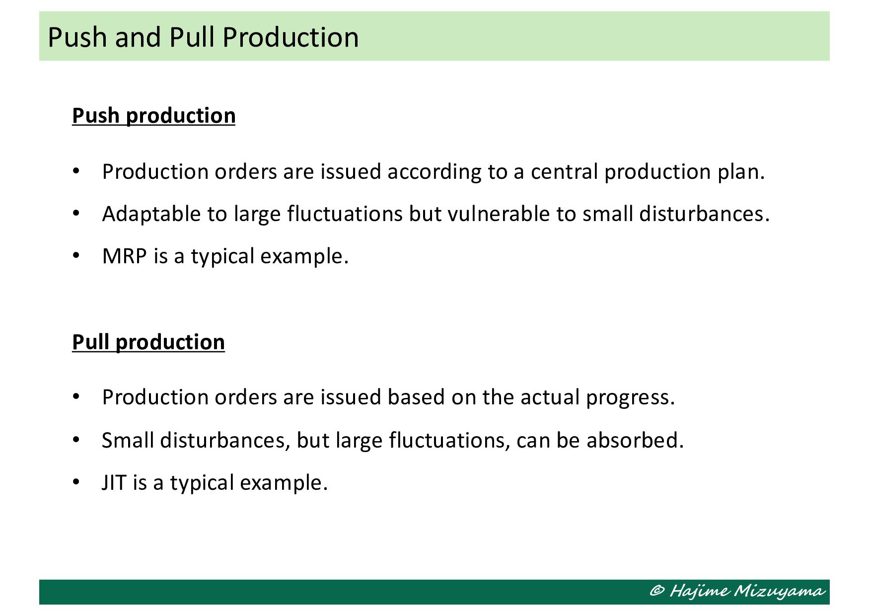
5. © Hajime Mizuyama Push production • Production orders are issued according to a central production plan. • Adaptable to large fluctuations but vulnerable to small disturbances. • MRP is a typical example. Pull production • Production orders are issued based on the actual progress. • Small disturbances, but large fluctuations, can be absorbed. • JIT is a typical example. Push and Pull Production
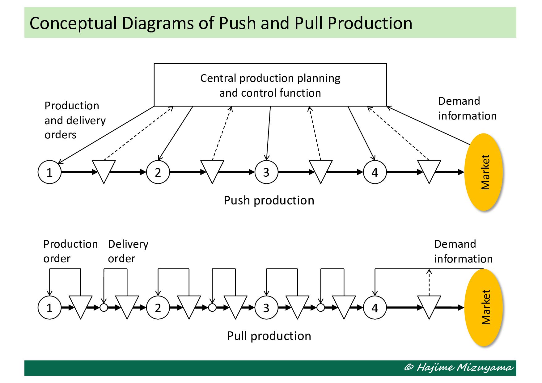
6. © Hajime Mizuyama Conceptual Diagrams of Push and Pull Production 1 2 3 4 Central production planning and control function Demand information Production and delivery orders Push production 1 2 3 4 Demand information Production order Pull production Delivery order Market Market
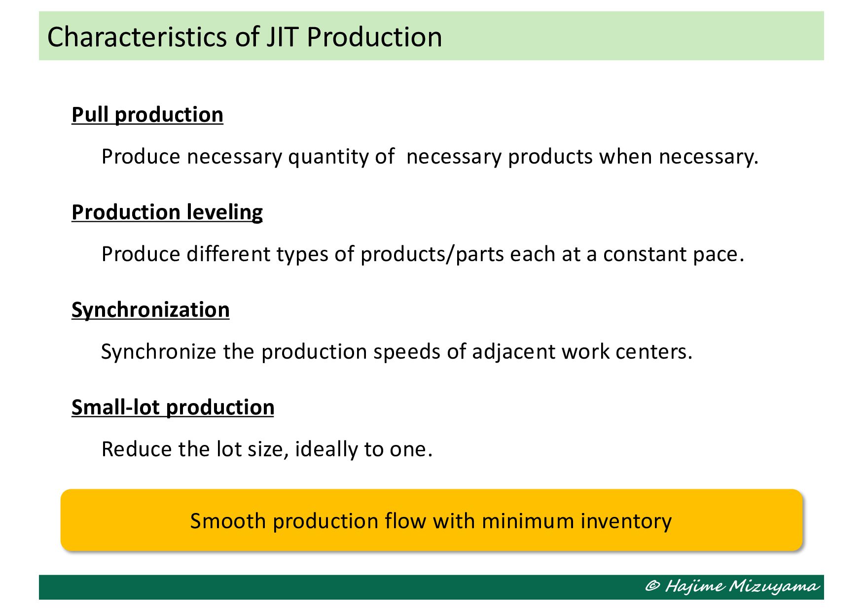
7. © Hajime Mizuyama Pull production Produce necessary quantity of necessary products when necessary. Production leveling Produce different types of products/parts each at a constant pace. Synchronization Synchronize the production speeds of adjacent work centers. Small-lot production Reduce the lot size, ideally to one. Characteristics of JIT Production Smooth production flow with minimum inventory
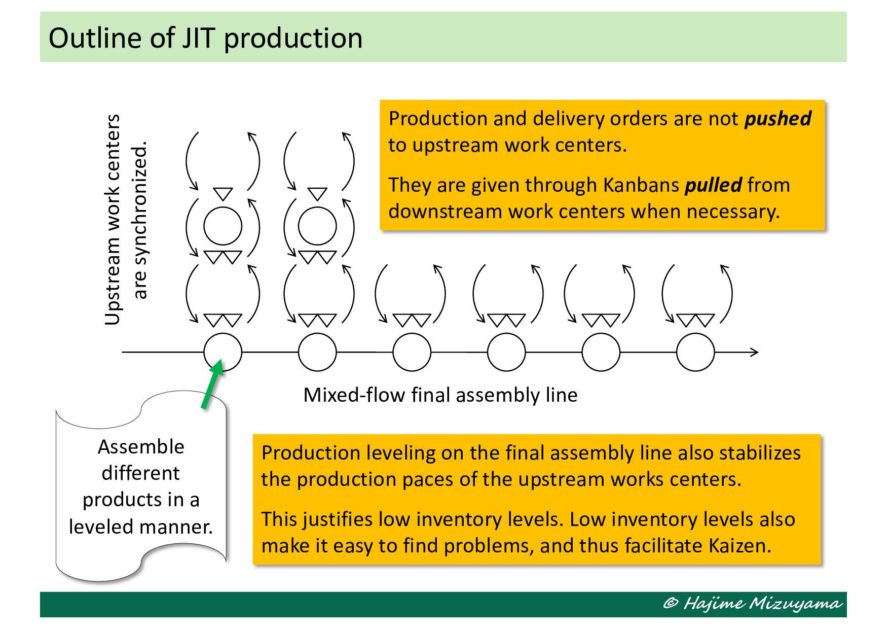
8. © Hajime Mizuyama Outline of JIT production Mixed-flow final assembly line Assemble different products in a leveled manner. Production and delivery orders are not pushed to upstream work centers. They are given through Kanbans pulled from downstream work centers when necessary. Production leveling on the final assembly line also stabilizes the production paces of the upstream works centers. This justifies low inventory levels. Low inventory levels also make it easy to find problems, and thus facilitate Kaizen. Upstream work centers are synchronized.
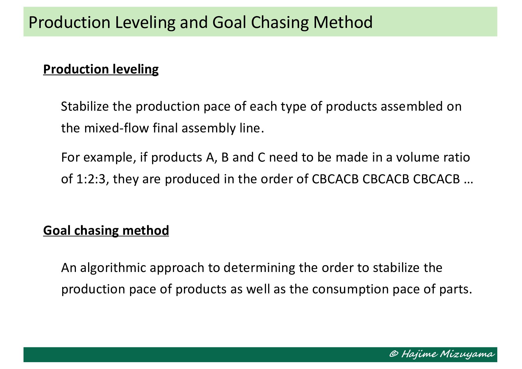
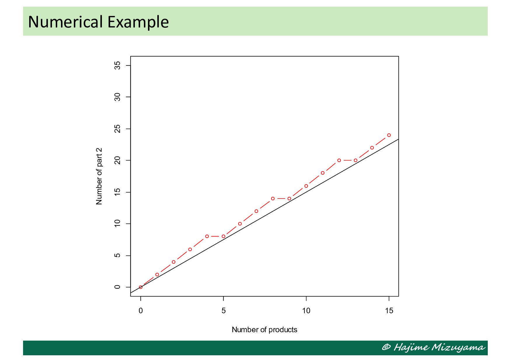
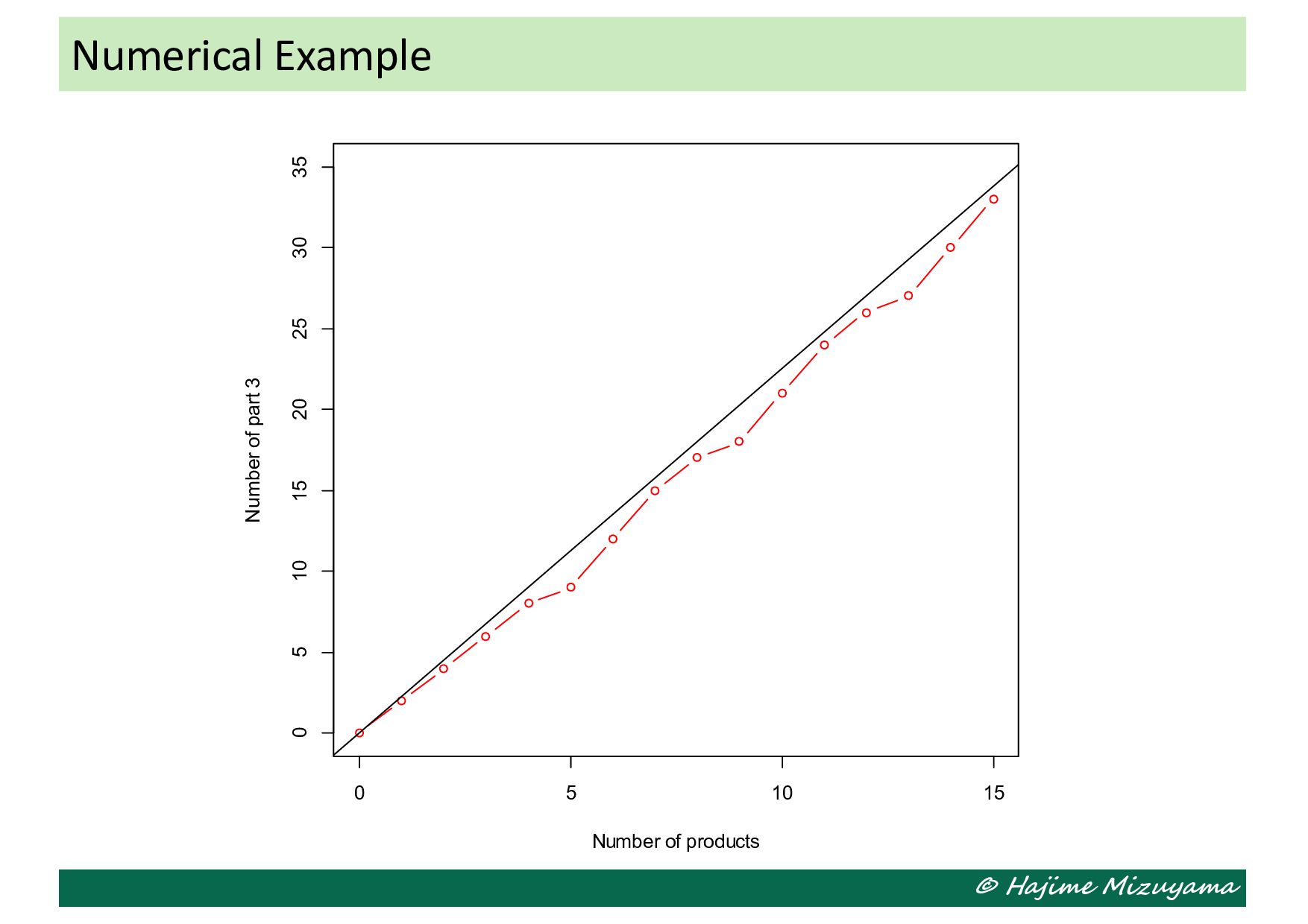
9. © Hajime Mizuyama Production leveling Stabilize the production pace of each type of products assembled on the mixed-flow final assembly line. For example, if products A, B and C need to be made in a volume ratio of 1:2:3, they are produced in the order of CBCACB CBCACB CBCACB … Goal chasing method An algorithmic approach to determining the order to stabilize the production pace of products as well as the consumption pace of parts. Production Leveling and Goal Chasing Method
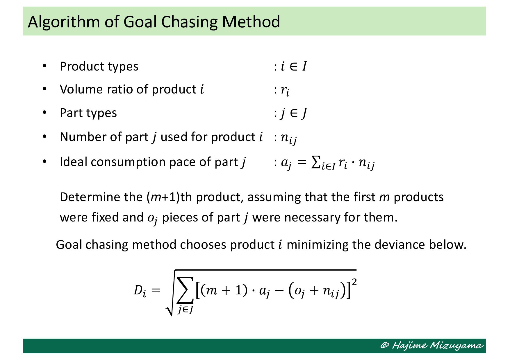
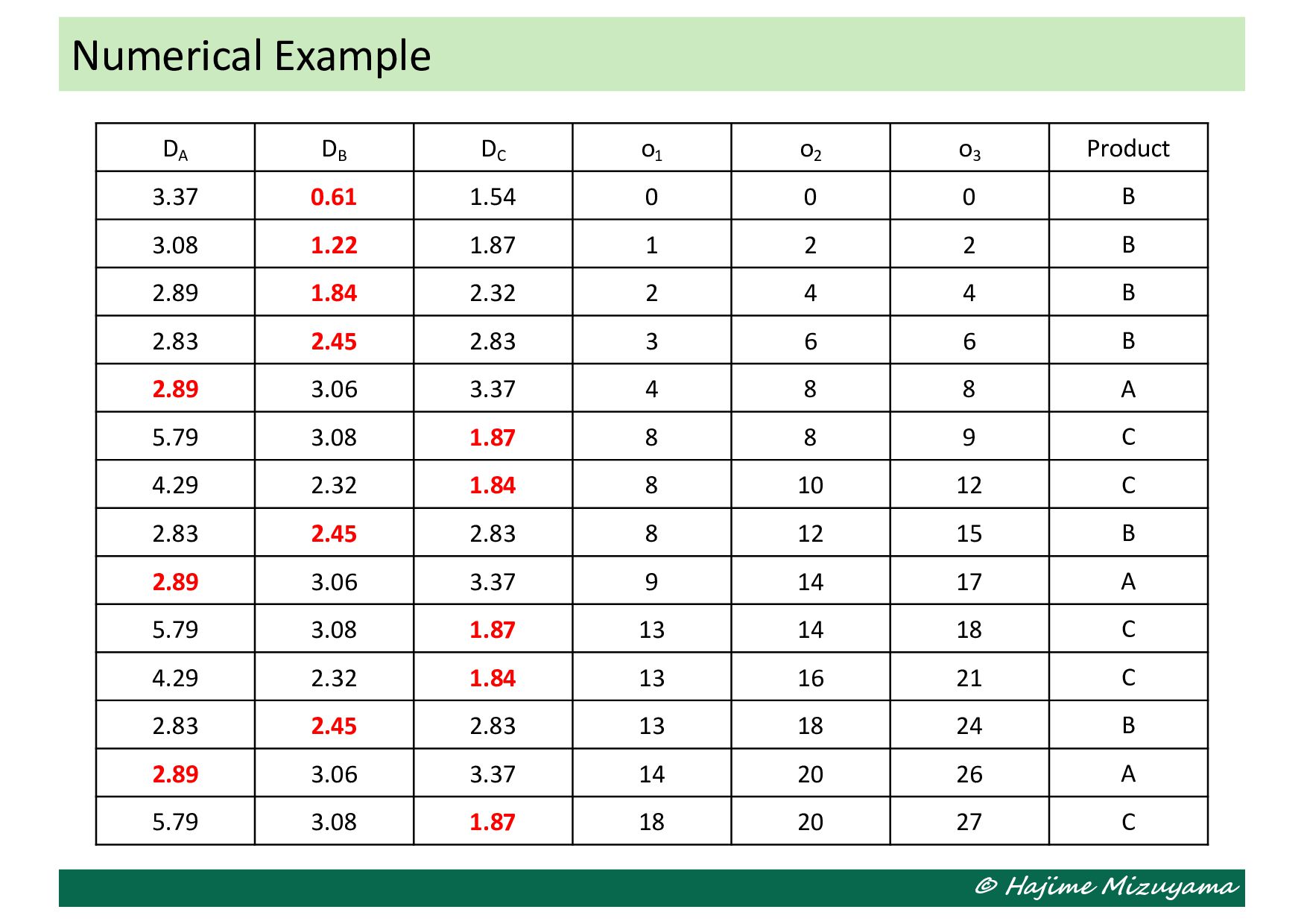
10. © Hajime Mizuyama • Product types : 𝑖 ∈ 𝐼 • Volume ratio of product 𝑖 : 𝑟! • Part types : 𝑗 ∈ 𝐽 • Number of part 𝑗 used for product 𝑖 : 𝑛!" • Ideal consumption pace of part 𝑗 : 𝑎" = ∑!∈$ 𝑟! + 𝑛!" Determine the (m+1)th product, assuming that the first m products were fixed and 𝑜" pieces of part 𝑗 were necessary for them. Goal chasing method chooses product 𝑖 minimizing the deviance below. 𝐷! = . "∈% 𝑚 + 1 + 𝑎" − 𝑜" + 𝑛!" & Algorithm of Goal Chasing Method
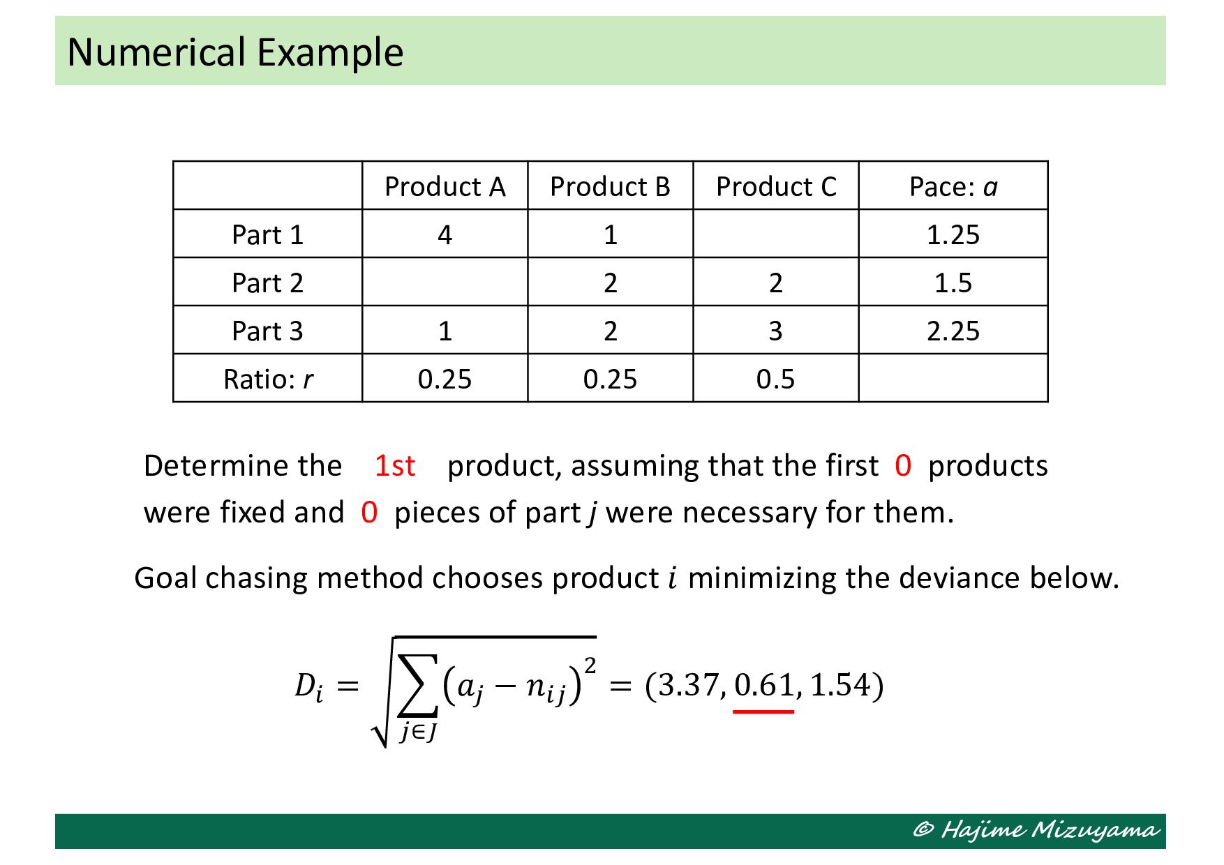
11. © Hajime Mizuyama Determine the 1st product, assuming that the first 0 products were fixed and 0 pieces of part j were necessary for them. Goal chasing method chooses product 𝑖 minimizing the deviance below. 𝐷! = . "∈% 𝑎" − 𝑛!" & = (3.37, 0.61, 1.54) Numerical Example Product A Product B Product C Pace: a Part 1 4 1 1.25 Part 2 2 2 1.5 Part 3 1 2 3 2.25 Ratio: r 0.25 0.25 0.5
12. © Hajime Mizuyama DA DB DC o1 o2 o3 Product 3.37 0.61 1.54 0 0 0 B 3.08 1.22 1.87 1 2 2 B 2.89 1.84 2.32 2 4 4 B 2.83 2.45 2.83 3 6 6 B 2.89 3.06 3.37 4 8 8 A 5.79 3.08 1.87 8 8 9 C 4.29 2.32 1.84 8 10 12 C 2.83 2.45 2.83 8 12 15 B 2.89 3.06 3.37 9 14 17 A 5.79 3.08 1.87 13 14 18 C 4.29 2.32 1.84 13 16 21 C 2.83 2.45 2.83 13 18 24 B 2.89 3.06 3.37 14 20 26 A 5.79 3.08 1.87 18 20 27 C Numerical Example
13. © Hajime Mizuyama Numerical Example 0 5 10 15 0 5 10 15 20 25 30 35 Number of products Number of part 1
14. © Hajime Mizuyama Numerical Example 0 5 10 15 0 5 10 15 20 25 30 35 Number of products Number of part 2
15. © Hajime Mizuyama Numerical Example 0 5 10 15 0 5 10 15 20 25 30 35 Number of products Number of part 3
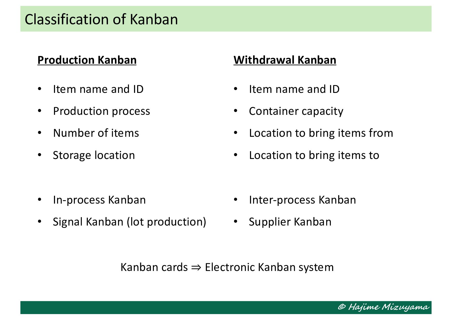
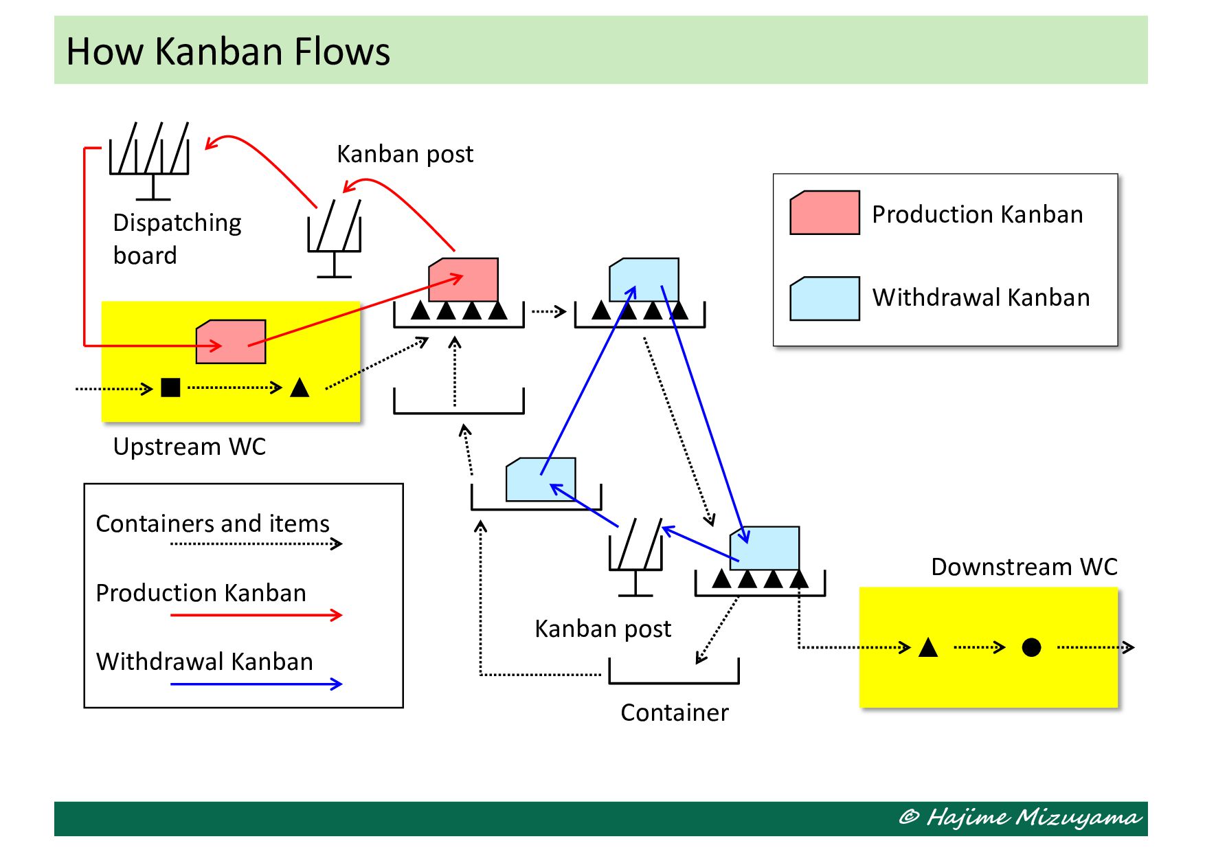
16. © Hajime Mizuyama Classification of Kanban Production Kanban • Item name and ID • Production process • Number of items • Storage location • In-process Kanban • Signal Kanban (lot production) Withdrawal Kanban • Item name and ID • Container capacity • Location to bring items from • Location to bring items to • Inter-process Kanban • Supplier Kanban Kanban cards ⇒ Electronic Kanban system
17. © Hajime Mizuyama How Kanban Flows Dispatching board Kanban post Production Kanban Withdrawal Kanban Withdrawal Kanban Kanban post Container Upstream WC Downstream WC Containers and items Production Kanban
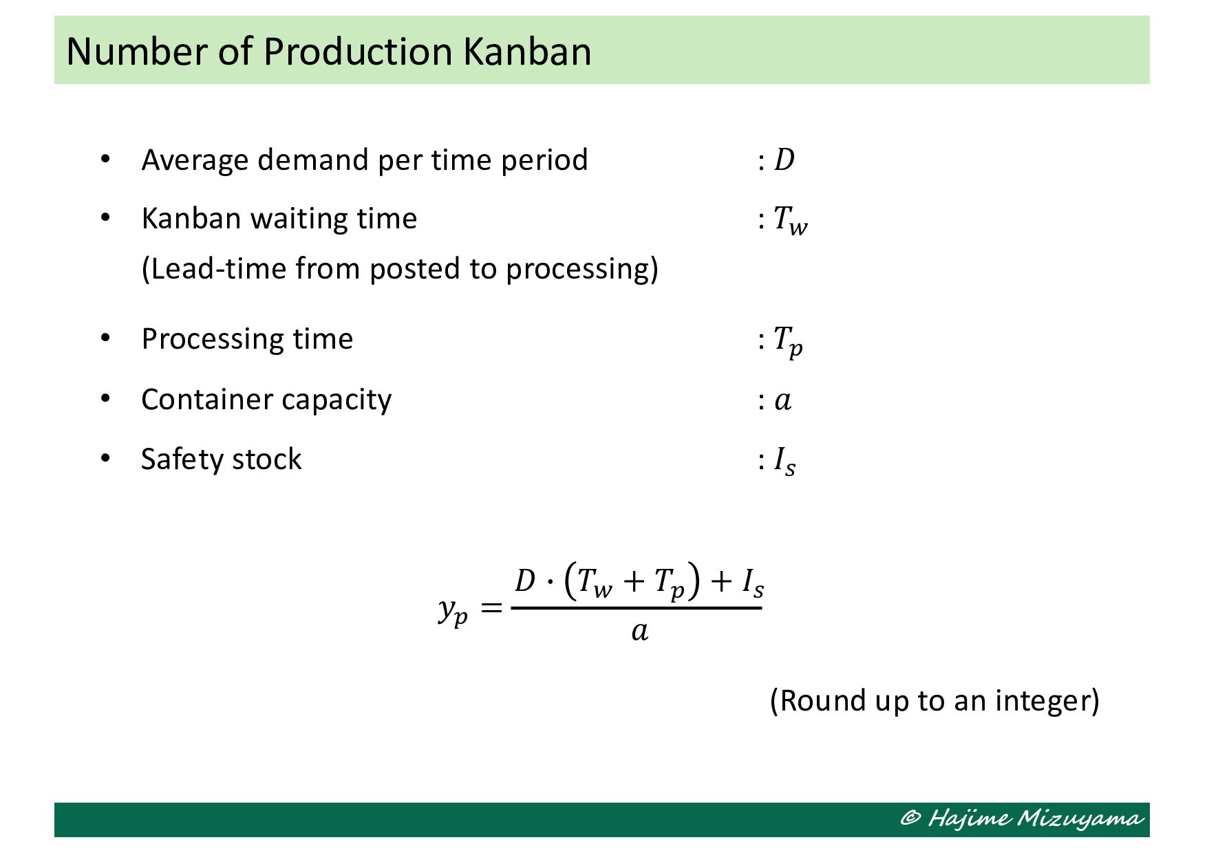
18. © Hajime Mizuyama • Average demand per time period : 𝐷 • Kanban waiting time : 𝑇' (Lead-time from posted to processing) • Processing time : 𝑇( • Container capacity : 𝑎 • Safety stock : 𝐼) 𝑦( = 𝐷 + 𝑇' + 𝑇( + 𝐼) 𝑎 Number of Production Kanban (Round up to an integer)
19. © Hajime Mizuyama • Average demand per time period : 𝐷 • Kanban waiting time : 𝑇' (Lead-time from posted to transporting) • Transporting time : 𝑇* • Container capacity : 𝑎 • Safety stock : 𝐼) 𝑦* = 𝐷 + 𝑇' + 𝑇* + 𝐼) 𝑎 Number of Withdrawal Kanban (Round up to an integer)